
How Full Is Too Full? Utilization, Queuing, and Microbursts
Sooner or later someone asks you the question directly: "at what percent should we worry about a link?" And somewhere in the back of your head, folklore answers for you: seventy. Keep links under 70% and you are fine; over 70% is the danger zone. It is one of the most repeated numbers in networking. And like most folklore, it is a real insight that fossilized into a rule, then outlived the world that made it true.
The honest answer is more interesting. A link can be genuinely troublesome at 40% average utilization and perfectly healthy at 98%. It depends on what kind of link it is and what rides on it. It also depends on what is happening inside the five-minute averages your graphs are made of. That is the part almost nobody teaches junior admins. The gap between "the graph looks fine" and "the users are suffering" is where this article lives.
By the end you will understand the two mechanisms that make links hurt before they are full — queuing delay and microbursts. You will know which counters betray problems your utilization graph cannot see. And you will have a table of practical starting thresholds per link type. Each starting threshold has the reasoning attached so you can adjust it instead of worshiping it.
In this guide
- Where the 70% folklore came from
- Queuing in plain words: why delay rises early
- What a 5-minute average can hide
- Microbursts: the 200-millisecond traffic jam
- The clues: drop and queue counters
- Different links, different rules
- Practical thresholds by link type
- When a link runs hot: the playbook
- Where to go next
Where the 70% folklore came from
The rule has two respectable grandparents. The first is ancient Ethernet. Early networks were shared media: every device on a segment shared one collision-prone channel, taking turns badly. On those half-duplex networks, useful throughput really did fall apart well before 100% load. That is because past a moderate utilization the devices spent more and more of their time colliding and retrying. "Never run Ethernet hot" was genuinely good advice — for a technology that modern switched, full-duplex networks retired long ago. A switch port today has the whole channel to itself in each direction; collisions are simply not a thing anymore. The rule survived the extinction of its reason.
The second grandparent is capacity planning. If a link trends at 70% during busy hours, it has little room left for growth or bad days. So 70% is a sensible start planning marker. That is a purchasing rule, not a performance rule. And folklore blurred the two into "past 70%, the network degrades," which is not what the planners meant.
So is 70% wrong? It is unearned. A dedicated backup link pinned at 98% all night is doing its job perfectly — congratulations, you sized it well. An internet edge carrying voice calls can be delivering robot-voice misery while averaging 45%. The percentage alone tells you neither story. To know when full is too full, you need to understand what fullness actually does to traffic — which is queuing.
Queuing in plain words: why delay rises early
A network link transmits exactly one packet at a time. When a packet arrives while another is being sent, it waits in a memory buffer — the queue. That is all congestion is: packets standing in line. The interesting part is when lines form, and the answer is: far earlier than intuition says, because traffic does not arrive politely spaced. It arrives in clumps.
Picture a supermarket with enough checkout capacity for the day's shoppers overall. Shoppers do not arrive evenly — they bunch. Even when the store is "half full," somebody is occasionally third in line. As the store fills toward capacity, the lines do not grow gently and linearly. They grow explosively, because every new clump of arrivals lands on a line that has not drained yet. At 95% of capacity the store still technically keeps up — and the lines are enormous.
Links behave the same way, and queuing theory gives the curve a memorable shape. A useful mental model for a steadily loaded link: the average wait is proportional to utilization ÷ (1 − utilization). Feed that formula and watch what happens. At 50% load the typical packet waits about one packet's worth of time. At 80% it waits about four; at 90% about nine. At 95% it waits about nineteen; at 99%, ninety-nine. The delay does not creep up — it turns a corner and climbs a wall. And the textbook version is the gentle case. It assumes smooth random arrivals, while real traffic is burstier, which bends the curve earlier and harder.
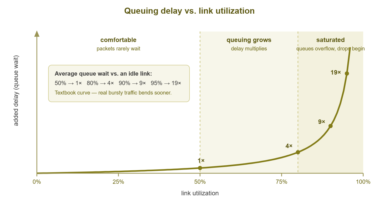
Figure 1: Delay versus utilization. The curve bends long before 100% — and real, bursty traffic bends it sooner than this textbook version.
Two conclusions fall straight out of the curve. First, "the link is not full, so the link is not the problem" is a fallacy. Delay damage starts in the 70s and 80s, and latency-sensitive traffic feels it first. Second, the last 10% of a link's capacity is not like the first 90%: traffic there pays for its bandwidth in waiting time. Whether that trade hurts depends entirely on what is waiting — a backup does not care about 40 extra milliseconds; a voice call absolutely does.
What a 5-minute average can hide
Now for the second mechanism, the one that makes calm-looking graphs lie. Standard monitoring reads interface counters every five minutes. A counter is an odometer, not a speedometer: it tells you how much traffic passed during the interval. And the graph point is the average rate across those 300 seconds. Everything about how the traffic was spread inside the interval is gone.
Run the numbers on a 1 Gbps link whose graph reads a soothing 40%. That means 15 GB moved in five minutes — but not when within them. Maybe it flowed steadily at 400 Mbps: healthy. Or maybe the link slammed to 100% for two full minutes of file transfer, then idled. That gives the same counter delta and the same graph point, but a very different afternoon for anyone sharing the link with the transfer. A link can run at line rate for 12 seconds out of every 300 and add just 4% to the average. Your graph literally cannot distinguish these worlds.
Shortening the polling interval helps less than you would hope. One-minute polls shrink the blur; they do not remove it, because the events that hurt real-time traffic are measured in milliseconds. No counter-polling cadence you can realistically run will see them directly. For that, you need to know what a microburst is.
There is still a sensible middle ground. During an active investigation, temporarily poll the one suspect interface every minute, or as fast as the device tolerates. You will not catch millisecond events. But you will often catch the two-minute slams that five-minute averages dissolve. The sharper graph narrows the window you ask flow data about. Just resist making hyper-fast polling permanent and universal. Frequent SNMP queries cost device CPU. And a monitoring system that stresses the network it watches has misunderstood the assignment.
Microbursts: the 200-millisecond traffic jam
A microburst is a surge that fills a link completely for a very short time — tens to hundreds of milliseconds. In that moment the output queue floods, latency spikes, and if the burst outlasts the buffer, packets are simply dropped. Then it is over, the queue drains, and the five-minute average absorbs the incident without a ripple. A 200 ms burst at 1 Gbps is only 25 MB — a single unremarkable chunk of a file copy. And that burst is 0.07% of a polling interval. Averaged over five minutes, it does not exist.
Microbursts are not freak events; they are the natural consequence of how networks are built. Three everyday causes:
- Speed mismatch. A server on a 10 Gbps port sends to a client behind a 1 Gbps uplink. The server can legally emit ten seconds of the slow link's capacity in one second. The switch between them has to queue the difference, and its buffer is finite.
- Fan-in. Twenty machines each send a modest flow toward the same uplink at the same moment. That might be a class opening the same shared folder or a backup kicking off across a rack. Individually trivial, simultaneously a wall of traffic converging on one port.
- TCP's rhythm. TCP deliberately probes for bandwidth by sending bursts within its transmission windows, ramping until loss tells it to back off. Even one healthy bulk transfer is a train of micro-surges by design.
Now consider who gets hurt. Bulk traffic barely notices a microburst: TCP retransmits the lost packets, throughput dips imperceptibly, the copy finishes a heartbeat later. But real-time traffic lives on a metronome. A voice call emits a packet roughly every 20 ms, and each must arrive on time to be played. Video conferencing is the same, faster. A 200 ms queue delays ten consecutive voice packets — audible as a garble or a dropout. A buffer overflow drops them unrecoverably. That is because by the time a retransmission could arrive, the moment it belonged to has already been played as silence. Voice and video apps do carry a small shock absorber — the jitter buffer. It holds a few dozen milliseconds of audio precisely so minor timing wobble goes unheard. But a 200 ms queue blows straight through it. This is the anatomy of the classic complaint: "calls keep breaking up, but the network graphs are fine." The graphs are fine. The milliseconds are not.
The clues: drop and queue counters
If polling cannot see microbursts, what can? Fortunately, the switch itself was there when it happened — and it kept a receipt. Every time an output queue overflows and a packet is thrown away, the interface increments a counter. That counter is output drops (in SNMP terms, ifOutDiscards). Drops are the fossil record of congestion too brief for your graphs. A device console will show something like this:
Interface Gi0/24  (uplink to core)
  5 minute output rate: 381 Mbit/s  (38% of 1 Gbps)
  Output queue: 0/1000 (size/max)
  Total output drops: 184223       <-- rising between checks

  Input errors: 0   CRC: 0   Output errors: 0
Read that carefully, because it is the signature: utilization modest, queue currently empty, errors zero — and a large, growing drop count. The link is fine on average and periodically getting slammed. The one number that matters is the trend. A static count may be ancient history (many counters only reset on reboot). So check it twice, twenty minutes apart. Or better, have your monitoring poll the discard counters alongside the traffic counters and alert on the rate of increase. Devices with quality-of-service configured usually expose per-queue drop counters too. Those add a bonus detail: they tell you which class of traffic is being sacrificed.
Tip: when the utilization graph and the drop counters disagree, believe the drops. The graph is an average taken over 300 seconds; the drop counter is an eyewitness that was present for every microsecond. A calm graph plus climbing output discards is not a contradiction — it is a diagnosis.
One caution in the other direction: drops are evidence of congestion, not proof of user pain. A bulk-only link can shrug off a modest drop rate — TCP is built for it. Drops plus real-time traffic, or drops plus complaints, is the combination that demands action. And near-zero drops on a busy link with tiny buffers does not fully acquit it either. But as first-line evidence goes, discard counters are the best microburst detector you already own.
Different links, different rules
We now have both mechanisms in hand: queuing delay rising early, and microbursts hiding inside averages. The folklore question finally gets a grown-up answer: it depends on the link's job.
User access ports (one PC, one port) are allowed to hit 100%. That is a person copying a file, and the port doing its job. Do not monitor them for utilization at all, except while troubleshooting that one user.
LAN uplinks and server ports are fan-in central: many access ports funnel into one uplink, which is exactly the microburst recipe. Sustained utilization here matters less than drops; plenty of LAN uplinks with modest averages quietly shed packets at every burst. Watch discard counters as seriously as percentages.
The internet edge is the expensive, shared, usually smallest pipe, and everyone's traffic meets there — so sustained busy-hour load genuinely predicts pain. On asymmetric circuits, remember the upload: it is the smaller direction, and it fills first. A saturated upload wrecks downloads too, because even downloads need a steady trickle of outbound acknowledgments to keep flowing.
WAN and site-to-site links carry the most latency-sensitive mix — voice, video, remote desktop, replication. Their queues are where the delay curve does visible damage first. These links justify the most conservative thresholds and are the strongest candidates for quality-of-service protection.
Dedicated backup and replication links invert the logic entirely: they exist to be filled. A backup link at 98% during its window is a success story. The alert-worthy condition is the window ending late, or the link running mysteriously idle when a job should be pushing it.
Practical thresholds by link type
These are starting points for sustained busy-hour utilization — the level a link holds during real working time, not one spike. Tune them to your network after a few weeks of baselines:
| Link type | Warn | Investigate | Reasoning |
|---|---|---|---|
| User access port | — | — | 100% is normal use; monitor only when troubleshooting |
| LAN / server uplink | 60% | 80%, or any rising drops | Fan-in makes microbursts likely well before averages look high |
| Internet edge | 70% | 85% | Shared by everyone; queuing delay grows steeply past the 70s |
| WAN / site-to-site with voice or video | 50–60% | 75% | Real-time traffic feels the delay curve first; headroom is the point |
| Dedicated backup / replication | — | Idle during window, or window overruns | Full is success; the failure mode is not full |
Two rules ride above every row of that table. First, any steadily rising output-drop counter is an investigation trigger regardless of percentage — the counters outrank the thresholds. Second, judge sustained load with an honest statistic: the busy-hour average or a 95th-percentile figure. Do not use the monthly average (which flatters) or the all-time peak (which panics). One freak spike is not a trend; every Tuesday at 80% is.
Warning: resist the urge to fix a threshold argument with more decimal places. The point of a warn level is to start a human looking before users hurt. The point of the reasoning column is to let you defend the number when someone asks. A threshold you cannot explain will be silenced the first week it annoys anyone — and then it protects nothing.
When a link runs hot: the playbook
A threshold fired, or the complaints did. Before anyone utters the word "upgrade," walk the sequence:
- 1. Verify the measurement. Check both directions — the busy one is often not the one on screen. Confirm on the device itself that you are seeing load, not sickness. Input errors and CRC failures mean a cabling or hardware problem that retransmissions then amplify into apparent congestion. Fixing a dying cable is cheaper than any circuit.
- 2. Characterize the shape. Sustained plateau through working hours, or spiky bursts with drops? The delay curve and the drop counters have already taught you these are different diseases — and they have different cures.
- 3. Identify the driver. A counter cannot name the culprit; flow data or the firewall's top-talker reports can. And one look usually sorts scheduled-job traffic from human traffic from waste.
- 4. Choose the lever. Now — only now — comes the real decision: buy more capacity, or manage the demand with scheduling, limits, and priority. That decision has its own guide: Upgrade or Shape? A Decision Framework for a Hot Link takes the evidence you just gathered and walks it to a defensible answer.
Where to go next
"How full is too full?" turns out to have a real answer — it is just not a single number. Delay climbs the queuing curve long before 100%. Averages hide millisecond-scale mayhem that drop counters faithfully record. And a healthy percentage on a backup link is a crisis number on a voice-bearing WAN. Watch busy-hour load against per-link-type thresholds, and watch discards always. Make the shape of the problem — sustained versus bursty — drive what you do next. The rest of Bandwidth & Utilization Monitoring picks up every thread from here. That includes measuring honestly, finding who is filling the pipe, and deciding what to do about it.
Put this into practice with SysPeep Monitor
Everything this guide asks you to watch is standard SNMP data. That includes per-link utilization in both directions, error counters, and the discard counters that betray microbursts. SysPeep Monitor discovers your interfaces, polls those counters on a schedule, and lets you set per-link thresholds with alerts. So the calm-looking graph and the climbing drop count land in the same dashboard. The free trial installs on a Windows machine in minutes.
Download Free TrialLearn About SysPeep - All Rights Reserved.