
How the Core Four Metrics Interact (and Mislead You)
Open any monitoring dashboard and you will find the same four graphs. First is bandwidth: how much data the link can move per second, and how much of that it is moving right now. The "how much" part is usually charted as utilization. Next is latency: how long one round trip takes, in milliseconds. Then comes jitter: how much that trip time wobbles from packet to packet. Finally, there is packet loss: the percentage of packets that never arrive at all. Each of the four has its own deep-dive guides in this library. This guide is about the thing the individual guides cannot show you: how the four behave together.
Because here is the trap. The dashboard draws four separate charts, so your brain files them as four separate facts — four independent dials you can read one at a time. They are not. All four are produced by the same underlying machinery, and they push and pull on each other in predictable ways. Read one graph in isolation and that machinery will cheerfully mislead you. It can lead you into blaming your ISP for a link you filled yourself. Or it can lead you into buying bandwidth to fix a loss problem. Or it can lead you into declaring a network "healthy" while every phone call on it sounds like a robot in a tunnel.
This guide teaches the six interaction patterns behind most of that confusion. For each one you will see what the graph shows, and what is physically happening underneath. You will see the wrong conclusion the graph invites you to draw, and the one quick check that settles the question. None of the checks needs special tools — a ping window and your interface graphs will do.
In this guide
- One mechanism connects all four: the queue
- Pattern 1: a filling link raises latency and jitter before loss
- Pattern 2: on TCP, loss disguises itself as low bandwidth
- Pattern 3: bufferbloat — giant buffers trade loss for latency
- Pattern 4: high latency caps TCP throughput on any pipe
- Pattern 5: jitter hides inside latency averages
- Pattern 6: real-time traffic breaks first
- The six patterns at a glance
- Where to go next
One mechanism connects all four: the queue
Picture a port on a switch or router as a checkout lane at a grocery store. The lane can scan a fixed number of items per second — that is bandwidth, the drain rate, a hard ceiling set by the hardware. Packets that arrive while the lane is busy do not vanish. They stand in line in a small chunk of the device's memory called a buffer (the line itself is called a queue). Every millisecond a packet spends standing in that line is added directly onto its latency. The line is longer in some moments than others, so the added wait keeps changing — and that variation is jitter. Finally, the buffer is finite. When the line is completely full, new arrivals are simply dropped on the floor. That — and on a healthy network, almost only that — is packet loss.
One mechanism, four gauges. This is why the metrics move together, and why they move in a particular order. As load on a link grows, you see utilization rise first, then latency, then jitter, and only at the very end, loss. The figure below walks through those four stages. Every pattern in the rest of this guide is a variation on this picture, so it is worth a long look.
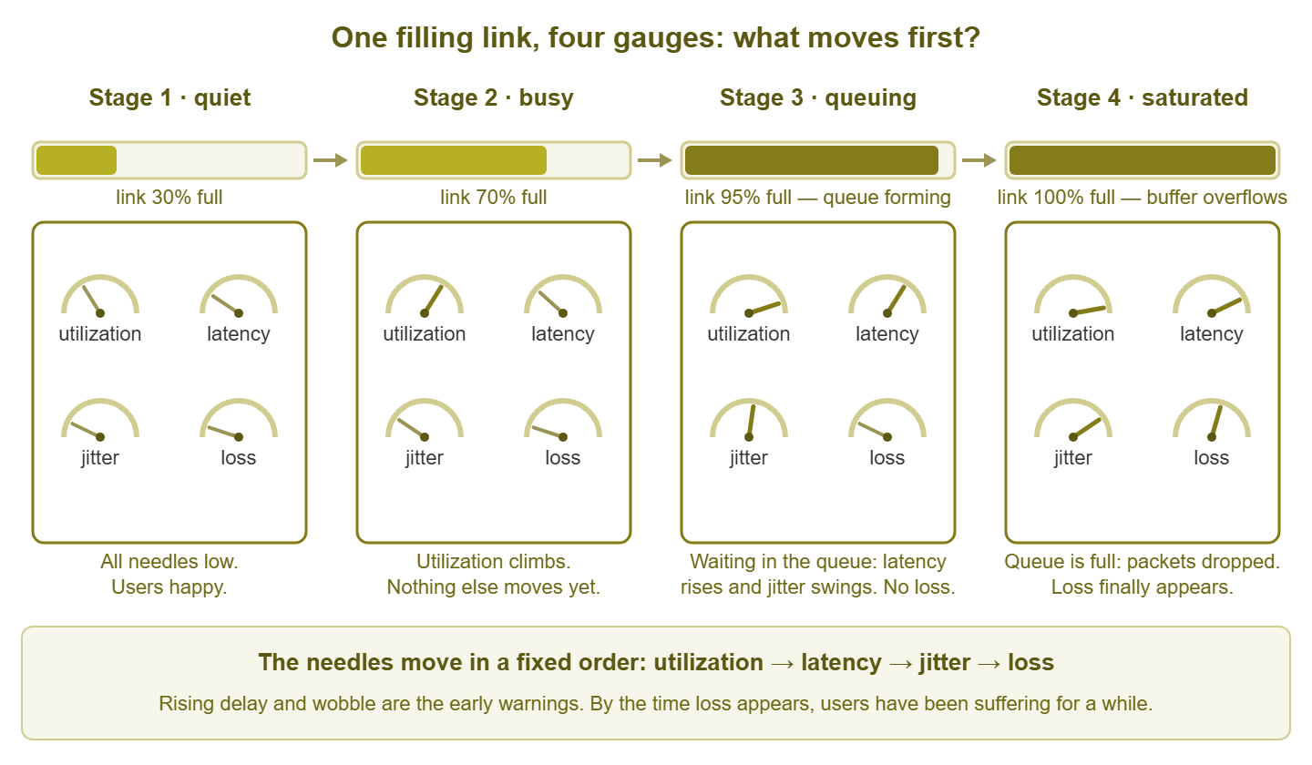
Figure 1: as a link fills, the four needles move in a fixed order. Latency and jitter are the early warnings; loss is the last resort.
Tip: queues only form under load, so the only latency measurement that tells you much is one taken while the link is busy. A clean ping test at midnight proves nothing about the 10 AM experience. Whenever a pattern below says "ping it," ping it during the pain, not after.
Pattern 1: a filling link raises latency and jitter before it drops anything
The story: an offsite backup job overruns into the workday and quietly fills the office uplink. At 9:15 the first tickets arrive — video calls stuttering, cloud apps "slow." You check the packet loss graph: a clean, reassuring zero. So the network must be fine… right?
What the graph shows: interface utilization climbing toward 100%. Ping times to anything beyond that link rising from their usual 20 ms to 60, 90, 120. The latency line turning visibly "furry" as it rises — that fur is jitter. And loss still flat at zero.
What is actually happening: the queue on the uplink is doing exactly what it was built to do. Packets are arriving faster than the link can drain them, so they wait. Every moment in the buffer lands straight on the latency graph. The depth of the queue changes from instant to instant as the backup's bursts come and go — which is precisely what jitter is. Nothing is dropped yet, because the buffer still has room. Queues are also sneaky about timing: delay grows gently while the link has headroom, then steeply as it approaches full. That is why a link can feel fine at 70% busy and terrible at 95%.
The misleading read: "loss is zero, so our line is clean — the ISP has developed a latency problem. Open a carrier ticket." The carrier tests the circuit, finds it flawless, and closes the ticket — because the circuit is flawless. The queue is yours, standing at your own doorway.
The check that settles it: put the utilization graph and the latency graph side by side on the same time axis. If latency rises exactly when utilization does, the delay lives in your own queue, not out on the internet. A live ping while it is happening shows the signature unmistakably:
Reply from 203.0.113.10: bytes=32 time=21ms TTL=55
Reply from 203.0.113.10: bytes=32 time=23ms TTL=55
Reply from 203.0.113.10: bytes=32 time=58ms TTL=55   <-- backup job kicks in
Reply from 203.0.113.10: bytes=32 time=84ms TTL=55
Reply from 203.0.113.10: bytes=32 time=112ms TTL=55  <-- queue is deep now
Reply from 203.0.113.10: bytes=32 time=67ms TTL=55   <-- and unsteady: jitter
Reply from 203.0.113.10: bytes=32 time=121ms TTL=55
Rising, wobbling times that track your utilization graph mean one thing. Find the flow that filled the link (interface graphs or top-talker views will point at it) and move it out of business hours. The latency "problem" will leave with it.
Pattern 2: on TCP, packet loss disguises itself as low bandwidth
The story: a branch office reports "the internet is slow." A speed test confirms it — 12 Mbit/s on a link rated for 100. The obvious conclusion, the one that writes itself into next quarter's budget, is that the branch has outgrown its circuit and needs a bigger one.
What the graph shows: low throughput. Transfers crawl, speed tests underperform, and utilization never gets anywhere near the link's rated capacity. Notice what is missing from the picture: nobody has said the word "loss." Unless you are deliberately measuring it, nothing on the screen says it either.
What is actually happening: somewhere on the path, a small percentage of packets is being discarded. That might be a failing patch cable, a speed/duplex mismatch, a dying optic, or an overloaded hop inside the carrier. TCP, the transport protocol underneath file copies, web pages, and most business traffic, hides that from users completely. It notices each missing segment and retransmits it, so no data ever actually goes missing. But TCP also treats every loss as a hint that the network is congested. So each drop makes the sender slow down sharply and then speed back up only cautiously. The result is a transfer that spends its whole life braking. The longer the path's round-trip time, the slower each recovery. That is why a loss rate too small to notice in a casual ping can cut throughput to a fraction of the line rate on a long path.
The misleading read: "we need more bandwidth." A bigger circuit fed through the same fault drops packets just as happily, and disappoints at a higher monthly price. Loss problems are never fixed by adding capacity; they are fixed by finding the drop.
The check that settles it: measure loss with enough samples to actually see it — a handful of pings cannot resolve a 2% problem. Run a few hundred (ping -n 200 203.0.113.10 on Windows) and read the summary, not the individual replies:
Ping statistics for 203.0.113.10:
    Packets: Sent = 200, Received = 195, Lost = 5 (2% loss)
Persistent loss above zero deserves a hunt: walk the path hop by hop and read the error and discard counters on every interface you control. Fix the drop, and the "bandwidth problem" evaporates without buying anything. The Packet Loss guides cover the hunt itself in detail.
Pattern 3: bufferbloat — giant buffers trade loss for latency
The story: a remote worker complains that whenever their cloud backup runs, their video calls collapse. You test their line: zero loss, and a speed test that hits the full advertised rate. Everything measurable says "healthy." The culprit has a memorable name: bufferbloat.
What the graph shows: latency to the user's site exploding under load — from a few milliseconds to several hundred — while packet loss stays pinned at zero. The instant the upload stops, latency snaps back to normal, as if nothing happened.
What is actually happening: some device on the path — very often a home or small-office router or modem — was built with an enormous buffer. Think back to the checkout lane: loss only happens when the line is full. Make the line absurdly long and it almost never fills, so nothing is dropped. But TCP relies on drops as its "please slow down" signal. Deprived of the signal, the sender keeps pushing until the giant buffer is permanently brim-full. Every packet from every application — including each tiny voice and video packet — has to wait through the entire line. The oversized buffer has converted what should have been brief, harmless loss into constant, crippling delay. It is a waiting room with no fire code.
The misleading read: "zero loss and a perfect speed test — the network is healthy, so the problem must be the app." In truth, those two clean readings are the fingerprint of the disease. The speed test looks great because the buffer never drops anything. Latency is terrible for exactly the same reason.
The check that settles it: start a continuous ping to a steady target, then saturate the link on purpose. A large upload is ideal, since the upstream side is usually the bloated one. If latency multiplies by ten or more while loss stays near zero, and recovers the moment the upload stops, that is bufferbloat. The fix is queue management, not capacity. Modern routers offer smart queue management (algorithms with names like CoDel and fq_codel) that keep the standing queue short on purpose. Even simple rate-shaping set just below the line rate moves the queue somewhere it can be managed.
Pattern 4: high latency caps TCP throughput — even on a fat pipe
The story: two sites are connected by a shiny new gigabit link. A single large file copy between them refuses to move faster than about 7 Mbit/s. Meanwhile the utilization graph shows the expensive new link sitting nearly idle. Nothing is broken and nothing is dropped. Distance is doing this.
What the graph shows: one transfer running far below the link speed; low utilization; a clean loss graph; and latency steady at, say, 70 ms round trip — entirely unremarkable for the distance between the sites.
What is actually happening: TCP is a polite protocol. It only allows a limited amount of data — called the window — to be "in flight" (sent but not yet acknowledged) at any moment. Once the window is used up, the sender stops and waits for acknowledgments. Acknowledgments take a full round trip to come back. So a single TCP stream can never move more than one window per round-trip time, no matter how enormous the pipe underneath it is:
max throughput of one TCP stream  =  window size / round-trip time

  64 KB window,  2 ms RTT (LAN):   64 x 8 / 0.002  =  ~256 Mbit/s
  64 KB window, 70 ms RTT (WAN):   64 x 8 / 0.070  =  ~7.3 Mbit/s

window needed to fill 1 Gbit/s at 70 ms:
  1 Gbit/s x 0.070 s  =  70 million bits  =  ~8.75 MB in flight
A classic 64 KB window at 70 ms mathematically cannot exceed about 7 Mbit/s. Modern operating systems scale windows far larger automatically. But plenty of things still pin them small: applications that set their own modest buffers, older protocol implementations, and middleboxes that interfere with window scaling. The pipe is fine; the sender is idling between permission slips.
The misleading read: "the carrier sold us a bad circuit" — or, more expensively, "we need ten gigabit." Extra capacity changes nothing when the limit is window ÷ round trip. The transfer would be exactly as slow on a link ten times the size.
The check that settles it: run several transfers in parallel. Each stream gets its own window. So if four streams together move roughly four times what one stream does, the path has plenty of capacity. In that case, you are looking at the per-stream window limit. Then do the arithmetic above: multiply the bandwidth you want by the round-trip time to get the window you need. Fix things at the endpoints — tuned buffers, more parallel streams, transfer tools built for long paths. And adjust expectations, because latency itself is set by geography. The Network Latency guides explain why no purchase order ever shortens a round trip.
Pattern 5: jitter hides inside latency averages
The story: the phone system generates complaints every morning — robotic voices, words dropping out mid-sentence. You pull up the latency graph for those exact hours: a serene, flat line at 24 ms. Case closed, network exonerated? Not yet. Jitter is latency's restlessness, and an average is where restlessness goes to disappear.
What the graph shows: average latency comfortably in range and no meaningful loss — while an application that depends on steady delivery is audibly suffering at the same moment.
What is actually happening: most monitoring polls a path every minute or five and stores an average of what it saw. Underneath that calm 24 ms average, individual packets are arriving after 10 ms, then 80, then 15, then 60. A queue somewhere is filling and draining in bursts. Real-time audio has to play at a fixed rhythm. So the receiving end smooths arrivals with a jitter buffer: a small holding area that delays everything slightly so playback stays even. Any packet that arrives later than the jitter buffer can wait is thrown away, exactly as if it had been lost. The average on your graph was true. It just was not the truth that mattered.
The misleading read: "latency is fine, so the network is fine — time to shout at the phone vendor." The average is fine. The variation is the problem, and an average is mathematically incapable of showing variation.
The check that settles it: look at the spread, not the middle. Graph the minimum and maximum response times alongside the average. A wide gap between those lines is jitter made visible. Better still, measure jitter directly. A UDP stream test (iperf3 in UDP mode, for example) reports it explicitly. Any continuous ping shows the wobble live in the time column. If your tools can only store averages, shorten the polling interval on the affected path so there is less room to hide.
Warning: an average hides everything shorter than the interval that produced it. A five-minute average can conceal a thirty-second disaster completely — and thirty seconds is an eternity in the middle of a phone call. When a graph and a user disagree, check what the graph averaged away before you doubt the user.
Pattern 6: real-time traffic breaks first — while bulk transfers look fine
The story: after a morning of "the calls sound like robots" tickets, somebody runs the classic test — copy a big file across the network. It flies. Hundreds of megabits. "Network's fine!" And yet the very next call sounds like a robot. Both observations are correct, because they are about two different networks that happen to share the same cables.
What the graph shows: throughput tests passing with flying colors, utilization looking moderate on the five-minute graphs, and a steady drip of real-time complaints that refuses to match either.
What is actually happening: a file copy and a voice call are opposite creatures. The copy uses large packets, tolerates any amount of delay and jitter, and retransmits its losses invisibly. It measures exactly one thing, how much the path can carry. The call sends a tiny packet every 20 milliseconds and needs each one to arrive on time. A late or lost voice packet cannot usefully be retried, because the moment it described has already been spoken. Short bursts of congestion — often caused by precisely the kind of bulk transfer being used as the "test" — delay or drop a few small packets at a time. The file copy sails through those bursts without noticing. The call audibly does not. And a five-minute utilization average flattens the bursts into invisibility, so the graph backs the wrong witness.
The misleading read: "the throughput test passed, so the network is healthy." A throughput test proves capacity. Real-time traffic barely consumes capacity — a phone call needs less bandwidth than the file copy wastes in rounding. It consumes punctuality: low loss and low jitter, which the test never measured.
The check that settles it: test with traffic shaped like the traffic that hurts. A small-packet UDP stream that reports loss and jitter, run during the problem window, stands in for a call far better than any file copy. On managed networks, also read the QoS (Quality of Service — traffic prioritization) queue counters on your switches and routers. Drops in the voice queue while the interface looks half idle are microbursts leaving fingerprints. The cure is prioritization and taming the bursty flows — not more bandwidth.
The six patterns at a glance
| Pattern | What you see | What is really happening | The fast check |
|---|---|---|---|
| 1. Filling link | Latency and jitter climb; loss still zero | A queue building at your own busy interface | Overlay utilization and latency; ping during load |
| 2. Loss on TCP | Low throughput; users say "slow" | Drops triggering retransmits and backoff | 200+ pings; error/discard counters along the path |
| 3. Bufferbloat | Huge latency under load; zero loss | An oversized buffer absorbing the overload | Ping while saturating the link; instant recovery after |
| 4. Latency caps TCP | One slow transfer on an idle fat link | Window ÷ round-trip limit per stream | Parallel streams; do the window math |
| 5. Hidden jitter | Flat average latency; real-time complaints | Spikes averaged away between polls | Graph min/max; run a UDP jitter test |
| 6. Real-time first | Throughput tests pass; calls break up | Small no-retry packets hitting bursts of delay and drop | Small-packet UDP probe; QoS queue drop counters |
Where to go next
Every pattern in this guide is the same queue wearing a different costume. Once you know the order in which the needles move — utilization, then latency, then jitter, then loss — you can read all four graphs as one story instead of four. Then the misleading conclusions lose their power. When a single metric deserves a closer look, the Network Latency and Packet Loss topics go deep on measuring and fixing each one. The rest of The Core Network Metrics covers what healthy values look like and which metric matters for which application. The full library lives at the topics index.
Put this into practice with SysPeep Monitor
Every pattern in this guide is easier to spot when the graphs sit side by side. SysPeep Monitor collects interface utilization, response times, and packet loss across your network over SNMP, WMI, and ping-style checks. It then puts them on one dashboard where a rising queue is obvious at a glance. It includes thresholds and alert rules that tell you before the tickets arrive. The free trial installs on any Windows machine in minutes.
Download Free TrialLearn About SysPeep - All Rights Reserved.