
Telemetry Explained: How a Counter Becomes a Chart
Right now, somewhere on your network, a switch is counting bytes. Somewhere on your screen there may be a chart of that port: a calm blue line you glance at before deciding the network is fine. That glance rests on a long chain of trust. The pixel is the last stop of a journey that began inside the switch's memory. At every stop along the way a little truth can quietly leak out. I have trusted that blue line and been wrong, and the line was never the part that was lying.
Telemetry means measuring things from far away — from the Greek tele (far) and metron (measure). Rockets send telemetry to mission control, race cars send it to the pit wall, and your switches, servers, and firewalls send it to your monitoring system. In IT the word covers the whole delivery pipeline. Numbers are collected from remote machines and shipped somewhere central so that a human, or an alert rule, can look at them. The rest of this guide is about what happens to a number in transit.
This guide follows a single number — the byte counter on one switch port — through every stage of that pipeline. The stages are exposure, collection, transport, storage, rollup, and rendering. At each stage you will see what happens, where accuracy can leak, and how to spot it. None of the leaks are scandals; each one is a reasonable engineering trade-off, made by someone sensible for a good reason. The only real danger is not knowing they exist. By the end you will read graphs with healthy suspicion, armed with questions that reveal more about any monitoring tool than its feature list ever will.
In this guide
- The traveler: one byte counter
- Stage 1: Exposure — a number you can ask for
- Stage 2: Collection — the poll cycle
- Stage 3: Transport — crossing the network
- Stage 4: Storage — becoming a time series
- Still stage 4: The rollup — history, compressed on purpose
- Stage 5: Rendering — rate math and the y-axis
- The leak map on one page
- Reading a graph backwards: a worked example
- The questions this lets you ask
The traveler: one byte counter
Our traveler is a counter: a number a device keeps that only ever goes up. The byte counter on a switch port works exactly like a car's odometer. It records the running total of every byte that has ever crossed the port since the device booted. It is not a speed. A single reading of an odometer tells you almost nothing; two readings, with the time between them, tell you how fast the car was going. Every bandwidth graph you have ever seen is built from that trick. Read the counter, wait, read it again, subtract, divide by the seconds in between. Everything that follows in this guide is about what can go wrong between the two readings.
On network gear this counter is exposed through SNMP (Simple Network Management Protocol, the standard question-and-answer protocol for network devices). The 64-bit version is named ifHCInOctets — octets being protocol-speak for bytes. On a Windows server the same kind of number is available through WMI (Windows Management Instrumentation, the operating system's built-in query interface) or from a small installed agent. Whatever the source, the pipeline ahead of it is the same, and it has five stages.
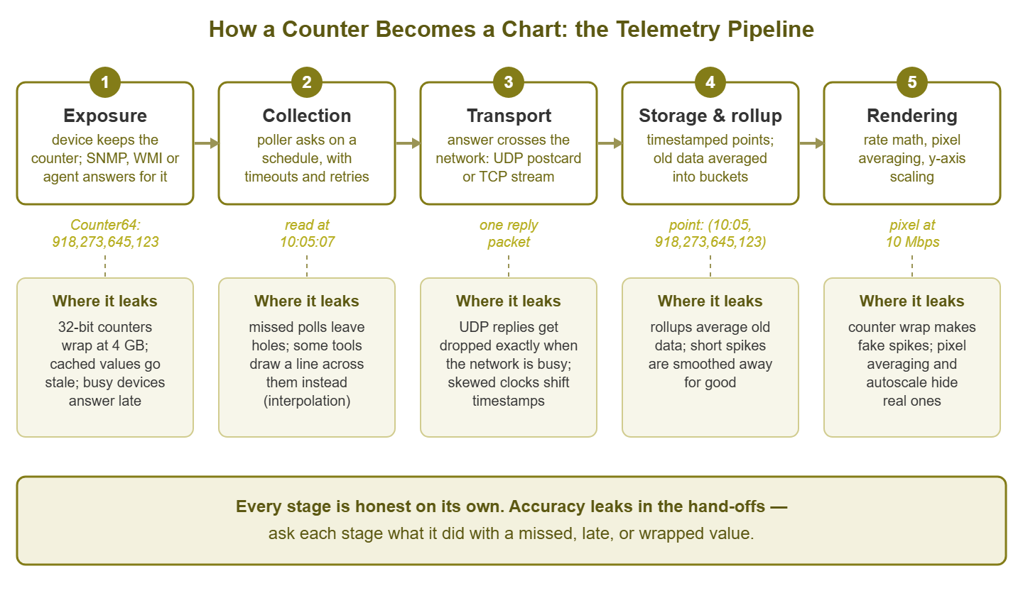
Figure 1: The telemetry pipeline. Every stage is honest on its own; accuracy leaks in the hand-offs between them.
Stage 1: Exposure — a number you can ask for
Deep inside the switch, the port hardware increments a register for every byte it forwards. That raw register is not what you query. A small program runs on the device — the SNMP agent, the WMI provider, or an installed monitoring agent. It periodically copies hardware registers into a table of values it is willing to share, and answers questions from that table. Exposure is this first hand-off: silicon to a nameable, askable number.
Where accuracy leaks: two ways. First, the agent's copy can be stale. Some devices refresh their SNMP counter table only every few seconds; ask twice quickly and you get the identical value, even though traffic flowed in between. Second, and more famous: counter wrap. Older 32-bit counters run out of digits at 4 GB and roll over to zero, exactly like an odometer passing 999,999. On a gigabit link running flat out, 4 GB takes about half a minute. So a counter polled every five minutes can wrap several times between readings. In that case, the subtraction produces confident nonsense. Reboots also reset every counter to zero, which makes naive math go negative.
How to spot it: stale caches show up as tiny staircases when you zoom far into a graph — flat ledges where values repeated. Wrap shows up as impossible spikes or sudden zeroes on busy links monitored with 32-bit counters. The fix for wrap is simply to prefer the 64-bit HC counters, which at gigabit speeds would take centuries to wrap. Check which one your tool actually reads, because that is a setting, not a law of nature.
Stage 2: Collection — the poll cycle
Your monitoring system keeps a work list: every device, every metric, and how often to ask — the polling interval, classically five minutes, often one. A scheduler walks the list, sends each question, and waits. Because devices are allowed to be slow, each question has a timeout (how long to wait for an answer, a few seconds). It also has a retry count (how many times to re-ask before giving up). Only after all retries fail does the poller record a miss. The poller is patient. It is one of the few things in the building that is.
Notice what this means for timing. A poll scheduled for 10:05:00 might get its answer at 10:05:00. Or — after one timeout and a retry — it might arrive at 10:05:09. Or the queue might be long and the question not even sent until 10:05:20. The reading is real, but when it happened is fuzzy. Rate math divides by elapsed time, so fuzzy timing bends the rate. Good tools record the actual moment of each answer and divide by actual elapsed time; weaker ones assume every gap is exactly one interval.
Where accuracy leaks: the missed poll. When a device fails to answer, the tool must decide what the chart will later show for that timeslot, and there are only three honest-ish options:
10:00  counter read OK
10:05  no answer (timed out after retries)
10:10  counter read OK

option A: store nothing        chart shows a visible gap
option B: interpolate          chart draws a straight line across the hole
option C: repeat last value    chart shows a suspicious flat ledge
Option A is the most truthful and the least pretty. Option B is interpolation: drawing a straight line between the two readings on either side of the hole. It looks professional and quietly invents data. The line implies traffic was average during a period when, very possibly, the device was too busy or too broken to answer. Option C is interpolation's stubborn cousin. None of these is wrong; charts full of holes have costs too. But know which one your tool does, because misses are not random noise. Devices go quiet precisely when overloaded. So the pipeline tends to fail during the exact minutes you will later care about.
How to spot it: find an outage you know happened and zoom into the graph. Gap, smooth line, or ledge? That is your tool's answer. Also glance at the poller's own health. If the monitoring machine cannot finish its work list within one interval, polls start slipping. In that case, every graph it draws gets subtly wobbly at once.
Tip: a graph with occasional visible gaps is often more trustworthy than one that never has any. The first tool is showing you its misses; the second may be papering over them. Absence of evidence, drawn as a straight line, starts to look like evidence.
Stage 3: Transport — crossing the network
The question and its answer travel the same network you are measuring, and the protocol underneath matters. SNMP normally rides on UDP (User Datagram Protocol), the postcard of network protocols: one packet out, one packet back, no delivery guarantee, no notification of loss. It is cheap and fast, which is why it scales to thousands of devices. Using UDP also means a congested network can silently eat the reply. Savor the irony: the measurement most likely to be lost is the measurement of the congestion that lost it. Installed agents and streaming systems usually push their data over TCP (Transmission Control Protocol) instead. TCP guarantees delivery by retransmitting. Nothing is lost, but data can arrive late, in bursts, after the connection recovers.
Where accuracy leaks: with UDP, silent loss — which the poller experiences as a timeout and handles as a missed poll. These misses cluster exactly around your busiest, most interesting moments. With TCP, delay raises a sneaky question. When a value arrives three minutes late, which timestamp gets stored, the moment it was measured or the moment it arrived? And whose clock supplies that timestamp? If the device stamps its own data and the device's clock is four minutes off, everything it reports is shifted four minutes against everything else. That is a lie so quiet you can stare straight at it during an incident review and not see it.
How to spot it: gaps that correlate with busy hours point at UDP loss. Events that seem to happen in the wrong order — the reboot that appears to follow the alert it caused — point at clock skew. Compare each device's clock against a common reference, and run NTP (Network Time Protocol, the standard clock-synchronization service) everywhere so the comparison stays boring.
Stage 4: Storage — becoming a time series
The answer arrives and is written down as a time-series point: which metric this is, a timestamp, and a value. A metric's history is just a long list of these points — that list is the "time series." Simple, but two storage decisions get made here that permanently shape the truth.
First: store the counter reading, or the rate computed from it? Many tools do the odometer subtraction immediately and store only the result — megabits per second — discarding the raw reading. That saves space, but it bakes this poll cycle's assumptions in forever. If a wrap or reboot fooled the subtraction, the wrong rate is now history, with no raw counter left to recompute from. Second: timestamps are usually snapped to tidy slot boundaries, which can slide a reading up to half an interval away from when it truly happened.
Where accuracy leaks: quietly baked-in rate errors, and small timestamp shifts. How to spot it: ask what is actually stored — readings or rates — and look at old history for preserved absurdities. A negative value, or a spike far above the physical speed of the link, is a wrap or reboot that got written down as fact. That error will now outlive us all.
Still stage 4: The rollup — history, compressed on purpose
Storage is where the pipeline's biggest, most deliberate accuracy trade lives: the rollup, also called downsampling or consolidation. The arithmetic that forces it is worth seeing once:
1 reading per minute              =      1,440 points per day
40 metrics on a device            =     57,600 points per device per day
200 devices                       = 11,520,000 points per day
one year of that                  = about 4.2 billion points
Nobody wants to buy disks for full-resolution eternity, and nobody wants to wait for a chart that reads a billion points. So almost every monitoring tool keeps recent data raw and periodically averages older data into bigger buckets. For example, a tool might keep one-minute points for a couple of weeks, five-minute averages for a few months, hourly or daily averages beyond that. The schedule varies; the idea is universal.
Averaging is a lossy compression, like shrinking a photo: the overall shape survives, fine detail is gone for good. And the detail that dies first is the spike:
what happened:      90 seconds at 950 Mbps, inside an otherwise quiet stretch
1-minute raw data:  two samples near 950 Mbps   (spike clearly visible)
5-minute average:   about 290 Mbps              (spike blurred)
1-hour average:     about 24 Mbps               (spike effectively gone)
Where accuracy leaks: the past smooths itself. The saturation event (a link running flat out at its full speed) everyone remembers becomes, a month later, a gentle bump. And if you do capacity planning (deciding how big the next link or disk needs to be) from long-term averages, you will size links for a calm network that never existed. Some tools soften the loss by storing the maximum alongside the average in each rollup bucket. If yours does, the max line is the one that remembers your bad days. How to spot it: look at the same incident this week and again after the rollup horizon passes. If the spike became a bump, you have seen your rollup policy at work. Then go read that policy, because it is configurable, and stretching raw retention for your dozen most important metrics is usually cheap.
Ashgrove Housing planned a WAN upgrade from a year of hourly averages, because that was the view the tool offered when you asked it for a year. The line peaked at a comfortable 30%, so the new circuit was sized with room to spare. On the first working day of the following month the rent run saturated it for twenty minutes. It had saturated the old circuit in exactly the same way on the first working day of every month. The hourly rollup had recorded that event each time as a gentle bump. The one-minute data that would have shown the ceiling had been rolled away after two weeks. The tool had kept the maximum alongside the average in every bucket, and nobody had ever clicked on it.
Stage 5: Rendering — rate math and the y-axis
Finally, the chart. If rates were not computed earlier, they are computed now, from pairs of stored counter readings:
later reading:     918,348,645,123 bytes
earlier reading:   918,273,645,123 bytes
difference:             75,000,000 bytes in 60 seconds
75,000,000 * 8 / 60 =   10,000,000 bits per second  =  10 Mbps
Two more quiet transformations happen at the last moment. First, pixel consolidation: a chart area maybe 700 pixels wide cannot show a month of one-minute data. That is over 43,000 points. So the renderer merges roughly 60 points into each pixel column, usually by averaging. This is a second rollup, performed live at display time, and it hides short spikes even when the raw data still contains them. Zooming in is not just magnification; it is un-averaging. Second, autoscaling: most charts stretch the y-axis to fit the data. A line wobbling between 49.9 and 50.1 Mbps, autoscaled, fills the chart with what looks like violent chaos. The same line on a 0-to-1000 axis is visibly, boringly flat. Autoscale manufactures drama out of jitter — the small, meaningless wobble every measurement has — and, zoomed the other way, flattens real trouble into wallpaper.
Where accuracy leaks: a spike your storage faithfully kept can still be invisible on screen. The emotional impression of a chart depends on an axis you did not choose. How to spot it: hover the line and read actual values instead of trusting shapes. Check whether the chart consolidates by average or by max. Some tools let you switch, and the views can differ dramatically. And when a graph looks alarming, read the y-axis numbers before your pulse does anything rash.
The leak map on one page
| Stage | The quiet leak | What it looks like | How to check |
|---|---|---|---|
| Exposure | Agent serves cached values | Tiny staircases at high zoom | Poll twice quickly; compare values |
| Exposure | 32-bit counter wraps at 4 GB | Impossible spikes or sudden zeroes | Confirm the tool reads 64-bit HC counters |
| Collection | Missed poll handled silently | Gap, invented straight line, or flat ledge | Find a known outage; zoom in; see which one |
| Collection | Polls slip when the poller is overloaded | Ragged timing, wobbly rates everywhere | Watch the monitoring server's own metrics |
| Transport | UDP replies dropped during congestion | Gaps clustered around the busiest moments | Compare gap times with busy hours |
| Transport | Clock skew between device and collector | Events in impossible order across sources | Audit clocks; run NTP everywhere |
| Storage | Rate stored, raw counter discarded | Wrap/reboot errors preserved as history | Ask what is stored; look for negative spikes |
| Storage | Rollups average old data | Last month's crisis is now a gentle bump | Read the retention policy; is max kept too? |
| Rendering | Many points merged per pixel | Spikes visible only after zooming in | Zoom; switch consolidation to max |
| Rendering | Autoscaled y-axis | Drama from jitter, or flattened trouble | Read the axis numbers before reacting |
Reading a graph backwards: a worked example
Monday morning, a user says Friday's big file transfers kept stalling around 9:15. You pull up the chart for the WAN link (wide area network — the circuit joining your sites) for the week. It shows a calm line that never crosses 40% — case closed, network was fine, must have been the application?
Not yet. Walk the pipeline backwards. Rendering first: the week view packs about fourteen minutes into every pixel. Zoom to Friday 9:00–10:00. The picture changes: a gap from roughly 9:05 to 9:20, then a tall block. Collection next: the poller's log confirms two consecutive poll timeouts for that device — the questions died in the very congestion the user felt. The chart's week view had quietly interpolated across the hole. Transport and exposure: the 9:20 poll succeeded and read the counter, which had kept honest count through the whole event. Now the odometer math tells the real story:
counter growth across the 15-minute hole:  67 GB
average the chart drew for that window:    67 GB * 8 / 900 s   =  about 600 Mbps
the server's transfer log shows ten calm minutes (~400 Mbps = 30 GB)
remaining 37 GB happened in 5 minutes:     37 GB * 8 / 300 s   =  about 990 Mbps
On a gigabit link, 990 Mbps is the ceiling. The link was saturated for about five minutes — the stalls were real. The pipeline hid it three separate ways. UDP polls were lost because of the congestion. The tool smoothed over the hole. And the surviving reading averaged five brutal minutes across a fifteen-minute window. No stage lied. The sum of their politeness was a chart that said "fine." Once you can run that backwards walk, no calm blue line will ever fully outrank a user who says something stalled.
The questions this lets you ask
You now understand telemetry plumbing well enough to interrogate any monitoring tool — commercial, open source, or the one you already run — with questions that have concrete, checkable answers:
- What happens to a missed poll — gap, repeated value, or interpolation — and how does the chart draw it?
- Do you read 64-bit counters when the device offers them, and how do you handle wraps and reboots?
- Which timestamp is stored — scheduled time, measurement time, or arrival time — and from whose clock?
- Do you store raw counter readings or only computed rates?
- What is the exact retention and rollup schedule, and do rollup buckets keep the maximum alongside the average?
- When a chart shows more points than pixels, does it consolidate by average or by max — and can I switch?
- Can I see and export the raw points behind any pixel I doubt?
A vendor or a tool that answers these crisply has thought hard about truth. Vague answers are information too. The same questions work on your own setup this afternoon. Pick one graph you rely on, and trace one pixel of it all the way back to a counter. It takes about an hour the first time, and afterwards the calm blue line is still calm. But it is no longer trusted on looks alone. The rest of the guides in Monitoring, Observability & Telemetry build on exactly this foundation — what the modern vocabulary means and how to grow a classic setup without replacing it.
Put this into practice with SysPeep Monitor
SysPeep Monitor runs this entire pipeline for you. It discovers the devices on your network, polls them over SNMP and WMI, stores the answers, and draws the dashboards. And now you know exactly which questions to ask of it, or of any tool. The free trial installs on a Windows machine in minutes. Bring the leak map along.
Download Free TrialLearn About SysPeep - All Rights Reserved.