
Rollups and Retention: How Monitoring Data Ages
Here is something your monitoring system probably never told you: it is quietly rewriting history. The detailed, minute-by-minute data it collects today will not exist in six months — not because of a bug or a crash, but by design. As samples age, the tool summarizes them into coarser and coarser form and throws the originals away. It is why last year's ugly outage looks strangely gentle when you pull up the old graph. It is also why the same week of data can tell two different stories depending on how far you zoom out.
This is not a scandal; it is a sensible bargain. Keeping every sample forever would drown your disk for the benefit of questions nobody asks. But the bargain has fine print. Admins who have never read it get burned in predictable ways. A spike "disappeared." An average hid the burst. An incident from March can no longer be investigated properly because March only survives as daily summaries.
This guide reads the fine print with you. It covers what a rollup actually is, the standard aging ladder almost every tool uses, and the storage math that justifies it. It also covers how to read old graphs without being fooled. And it shows how to adjust the ladder so it keeps what you will need. By the end you will know exactly what your history can and cannot testify to — before you need its testimony.
In this guide
- What a rollup actually is
- The standard aging ladder
- The storage math that justifies it
- What aging does to different kinds of metrics
- Reading rolled-up graphs honestly
- The forensic implication: can you still see last Tuesday?
- What each rung can still answer
- Your ladder is configured, not fated
- The retention-ladder audit
What a rollup actually is
A rollup (some tools say consolidation, aggregation, or downsampling) is many fine-grained samples summarized into one coarse data point. Take an interface's utilization, polled every minute. After some weeks, the tool takes each hour's sixty samples and replaces them with a single hourly value. Sixty numbers in, one number out, fifty-nine numbers gone forever. Do that for every hour, and a week of data shrinks from 10,080 points to 168.
The crucial detail is which one number survives. For each window the tool can keep the average (what the value typically was), the maximum (the worst moment), or the minimum. Or it can keep several of these side by side. Tools differ, and this is the single most important thing to learn about yours: does your rollup keep the max? If a rollup keeps only averages, then every spike shorter than the rollup window is erased forever — not hidden, not compressed, erased. The hour when a link hit 95% for ten minutes becomes "40%". No amount of zooming, exporting, or wishful clicking will ever bring the 95% back. A rollup that also keeps the per-window max preserves at least the fact that a worst moment happened and how bad it was. It preserves that even after the shape of it is gone. Averages tell you what was normal; maxima remember what went wrong. You want both.
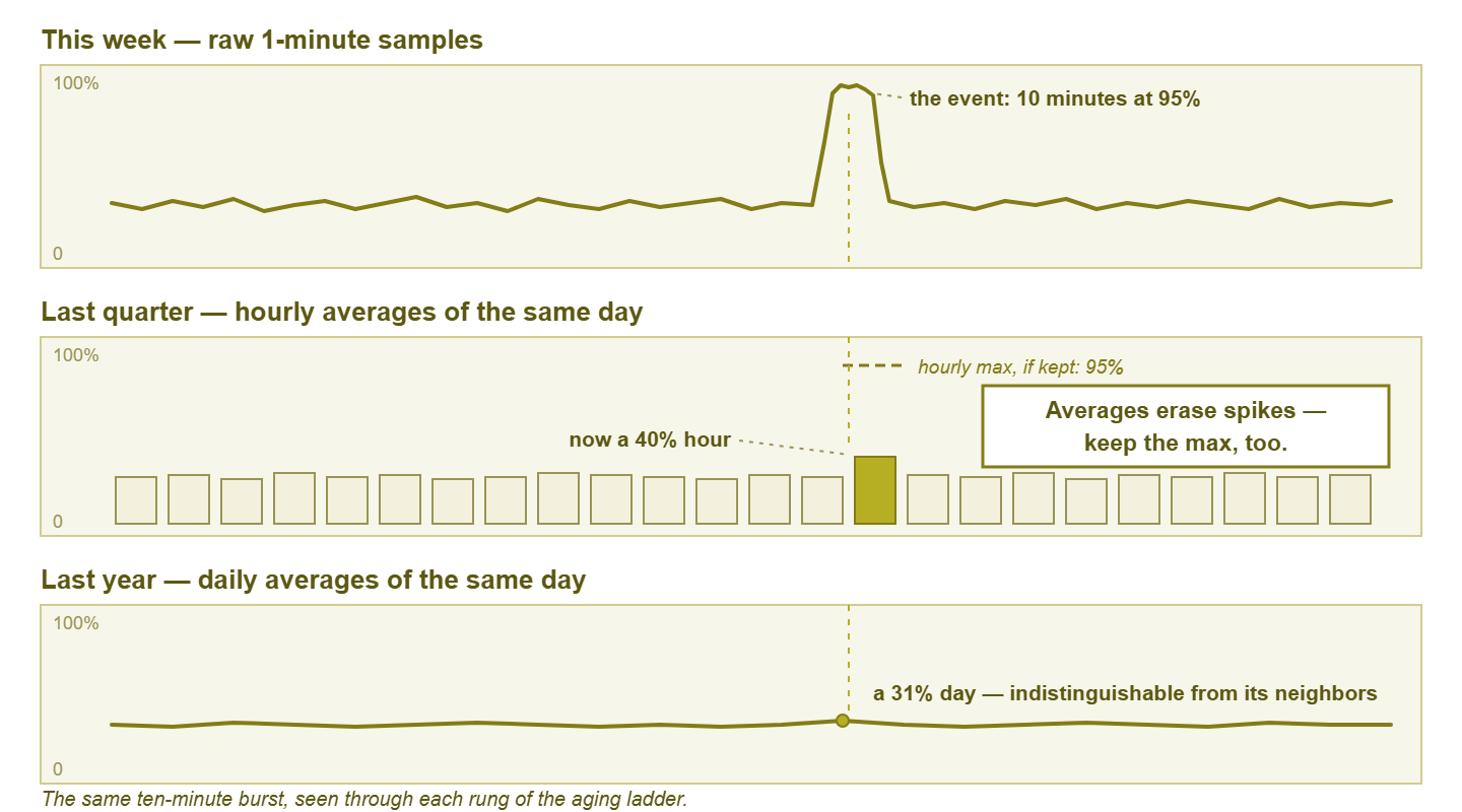
Figure 1: the same ten-minute burst, seen through each rung of the aging ladder. In averages-only rollups, the oldest view is all that remains.
The standard aging ladder
Nearly every monitoring tool ages data down a ladder. It keeps raw samples at the polling interval for a short window. Then come progressively coarser summaries for progressively longer spans. The steps and spans vary by product, but the shape is remarkably universal — something close to this:
| Rung | Resolution | Typical span kept | What survives on this rung |
|---|---|---|---|
| Raw | Native polling interval (e.g. 1–5 min) | Days to a few weeks | Everything the poller saw: real shape, real spikes, real gaps |
| Fine summary | 5–15 min per point | Weeks to a couple of months | Shape of busy periods; short spikes already blurring (max, if kept, still flags them) |
| Hourly | 1 hour per point | Months to a year | Daily rhythm and trends; anything shorter than an hour is a faint dent |
| Daily | 1 day per point | Years | Long-term growth and seasonality; individual events effectively gone |
Under the hood, tools implement the ladder in one of two ways. Some use fixed-size round-robin archives. Each rung is a ring of slots, new points overwrite the oldest, and disk usage never grows — tidy. But the spans are decided up front. Others store samples in a database and run background jobs that periodically summarize aged rows and delete the originals. That is flexible, but the deletions are real and scheduled, whether or not you were finished with the data. Either way the aging is automatic and silent. No dialog box will ever ask whether you still needed last month at full resolution.
Each rung answers coarser questions than the one above it, and the handoffs are where detail dies. The ladder is not good or bad in itself — it is a default someone chose for the average customer. Whether it fits your investigations and your reporting is the question the rest of this guide equips you to answer.
The storage math that justifies it
Why do tools bother? Multiply three numbers, same as every capacity question in monitoring. Suppose a modest estate: 100 devices, 30 metrics each, polled every minute. That is 3,000 samples per minute — about 4.3 million samples per day, roughly 1.6 billion per year. At a few tens of bytes per stored sample (value, timestamp, indexing overhead), a year of raw data lands in the tens of gigabytes. Not apocalyptic on modern disks — but growing forever, competing with backups for space, and slowing every query that has to wade through it. Meanwhile the hourly-summary version of the same year is sixty times smaller, and the daily version is over a thousand times smaller.
And here is the honest kicker: almost nobody queries eleven-month-old data at one-minute resolution. The ladder spends storage where queries actually go — fine and recent, coarse and old. It is the same economics that governs flow records, where the multiplication is even scarier. The flow storage math guide runs those numbers. The shape of the answer is identical: keep detail briefly, keep summaries long, and decide the crossover on purpose.
What aging does to different kinds of metrics
The ladder treats every metric the same way, but metrics are not all the same kind of number, and it pays to know how each kind ages.
Gauges: the straightforward case
A gauge is a metric that reads as a level at an instant — CPU percent, temperature, disk fill, connection count. Rollups do to gauges exactly what this guide has described. Averages describe the typical level, maxima remember the worst one, and short excursions dissolve unless a max is kept. Everything above applies verbatim.
Counter-derived rates: already averages before they age
Traffic and error metrics usually start life as counters — ever-increasing tallies on the device (total bytes sent, total errors). Your tool converts them to rates by subtracting successive readings and dividing by the time between polls. That means a "1-minute traffic sample" is already an average over that minute before any rollup touches it. Sub-minute bursts were smoothed at birth. Rollups then average the averages. There are two lessons. The raw rung is as sharp as this data ever gets, so guard it for the metrics you investigate. And the burst-blindness of rate metrics is a polling phenomenon, not just a retention one. The guide to what your polling interval cannot see takes that thread further.
Up/down state: aging into percentages
Availability checks age differently again. A stream of up/up/down/up samples cannot be "averaged" as numbers. So tools typically summarize state history into percent available per window — and sometimes keep an event log of transitions alongside. Once the raw samples are gone, a three-minute outage on a Tuesday survives only as "99.8% that day." That proves something happened but no longer says when, or whether it was one blip or three. If you owe anyone uptime reporting, check whether your tool preserves the outage events long-term or only the percentages. The difference decides whether next year you can answer "which afternoon was that?" or only "roughly how bad was the quarter?"
Gaps: the samples that never existed
Finally, missing data. When the poller was down, the WAN was cut, or a device was unreachable, there are simply no samples for that stretch. In the raw view most tools draw an honest hole. But as data ages, a window containing gaps gets summarized from whatever samples do exist. The hole quietly heals over. An hour with twenty minutes of missing data becomes an ordinary-looking hourly point computed from the other forty. Old graphs are therefore smoother and more complete-looking than the collection ever was. When an old chart of a flaky period looks suspiciously serene, ask what the poller was doing at the time before you believe it.
Reading rolled-up graphs honestly
Now the practical skill: not being fooled by your own charts. When you widen a graph's time range, most tools silently switch to a coarser rung of the ladder. The six-hour view draws raw samples, the three-month view draws hourly averages, and the two-year view draws dailies. Same metric, same pixels, different testimony. The result is the zoom-level effect: a spike that shrinks as you zoom out, then vanishes.
Watch it happen with real numbers. A link runs at a calm 29% for fifty minutes of an hour, but bursts to 95% for ten minutes. Users notice. Someone files a ticket. In the raw view, there it is: a sharp tower to 95%. Zoom to the quarter view, drawn from hourly averages. Ten minutes of 95 and fifty minutes of 29 average to 40%. Your crisis is now a mild bump. Zoom to the year view, drawn from daily averages. One busy hour dissolves into 23 ordinary ones and the day reads about 31% — indistinguishable from the day before. Nothing was deleted between your first look and your last (yet). The graph simply answered a different question at each zoom: "what happened?", then "what was typical per hour?", then "what was typical per day?"
Two habits make you immune. First, the rule: judge an event at the finest granularity that still covers it. Investigating something from yesterday? Insist on the raw view. From last quarter? The hourly rung is the best testimony that still exists — and read its maxima, not just its averages, if you have them. Second, know what you are looking at: check what resolution the current view is drawn from. Some tools display it ("avg per point: 1 h"). In others you infer it by counting. A one-month graph drawn with thirty visible steps is daily data wearing a smooth line. Never let a wide, gentle graph talk you out of an event that a narrow view — or a user — reported. The graph is not lying; it is summarizing, which at the wrong zoom level is the same thing.
Tip: when you screenshot a graph for a ticket, a postmortem, or your boss, capture the zoomed-in raw view of the event, not the roomy month view. Months later, the raw rung will be gone and that screenshot may be the only full-resolution witness left. It costs one extra click today and it has saved many an argument.
The forensic implication: can you still see last Tuesday?
Rollups turn retention into a forensic question. An incident older than your raw window can only ever be examined through summary glasses. Whatever rung it has aged onto is now the finest truth available. If your raw window is seven days and the weird slowdown happened twelve days ago, you will investigate ten-minute phenomena with hourly averages. That is like reconstructing a conversation from the meeting minutes.
So set the raw window from your investigation habits, not from the tool's default. The test is concrete: "Can I still see last Tuesday properly?" Think about how late problems actually reach you. A user mentions "it's been slow for a while" two weeks after it started. A monthly review spots something odd from the 3rd. You only correlate an intermittent fault after its third occurrence. In most small shops that argues for two to six weeks of raw data, not the few days some defaults ship with. Storage is the cheapest ingredient in an investigation; the question you cannot answer anymore is the expensive one.
One more forensic habit: when an investigation is going to outlive the raw window, export the raw data now, while it exists. Think of the intermittent fault you are stalking across weeks, or the dispute with a provider that lawyers might eventually enjoy. A CSV export or a saved report of the relevant series is a permanent, full-resolution witness that no rollup job can touch. The ladder ages what is in the database; it cannot age what you copied out of it.
What each rung can still answer
Retention serves needs, so match the rungs to the questions you actually ask of history:
- Alerting barely touches history at all — it evaluates fresh samples as they arrive, so no rollup choice can hurt your alarms. (Alert tuning is another story: picking good thresholds means studying recent behavior, which wants the raw rung.)
- Troubleshooting and forensics want raw, full stop — this is the need that sizes your raw window, as above.
- Baselining — building the recorded picture of "normal" — lives happily on the fine-summary and hourly rungs. It is about typical patterns, and summaries are typical patterns. A year of hourly data is a superb baseline substrate; the collecting baselines guide shows what to do with it.
- Capacity planning is happiest of all on dailies. "How fast is this filling and when does it hit the wall" is a months-scale question. Daily points for two or three years answer it better than any amount of minute data. Keep per-day maxima alongside averages and you can plan for peaks, not just for averages.
- Reporting and SLA evidence mostly needs availability history and coarse performance summaries over long spans. Dailies with honest maxima usually suffice, but check what your reports promise before the ladder eats the proof.
Your ladder is configured, not fated
Every tool ships a default ladder. The default is a guess about an average customer — sized to flatter the tool's disk usage, tuned for nobody in particular. Somewhere in your tool's settings, the rungs and spans are spelled out, along with which aggregates each rung keeps. Look for "data retention," "history," "consolidation," or "storage" options. Go find yours; it is a five-minute errand that most admins have never run.
Then adjust it per metric class, because uniform retention is as lazy as uniform polling. High-value metrics earn longer raw windows: the WAN links, the firewall, the latency checks on the money path — the places where investigations happen and evidence matters. Bulk metrics — the lab gear, the per-port stats on access switches — can age quickly onto coarse rungs with a clear conscience. If your tool only offers one global ladder, set it for your most demanding class and accept the overspend on the rest. Disk is cheaper than a missing answer.
The retention-ladder audit
Close the loop with a half-hour exercise that turns all of this from theory into settings:
- 1. Find your ladder. Locate the retention settings and write down each rung: resolution, span, and which aggregates (average? max? min?) it keeps. If it is averages-only, you have found this audit's headline.
- 2. Test the zoom effect on a known event. Pick an incident you remember — a saturated link, a hot CPU day. View it at raw, then at the wider zooms, and watch it shrink. Note the age at which it stops being visibly an incident. That age is your real forensic horizon, measured, not assumed.
- 3. Adjust one class deliberately. Lengthen the raw window on your handful of high-value metrics to cover your honest investigation lag. Enable max-keeping if it is off, and note the projected disk change. One deliberate adjustment beats a policy document nobody wrote.
Step three, scaled up and written down, becomes a real retention policy — classes, ladders, exceptions, and a storage projection on one page. That is the next guide: a metric retention policy for small shops. And for the rest of the story of how sampling shapes what you can know — intervals, load, and blind spots — the Polling Intervals & Data Granularity pillar has the map.
Put this into practice with SysPeep Monitor
Retention tuning is easier when you can see and steer where the data lives. SysPeep Monitor stores its history in your choice of SQLite, MySQL/MariaDB or SQL Server. Its dashboards and reports let you inspect a metric's history at the resolution you need. The free trial installs on any Windows machine.
Download Free TrialLearn About SysPeep - All Rights Reserved.