
Smokeping-Style Latency Graphing
Somebody says the network is "slow sometimes." You ping the server. Four tidy replies come back at 12 milliseconds. You type the least satisfying sentence in IT: "it looks fine from here." Here is the frustrating part — you are both right. The network really is misbehaving sometimes, and it really is fine right now. A ping is a snapshot. The problem is a movie, and it has no intention of performing while you are watching.
Smokeping-style latency graphing closes that gap. The idea is simple and a little relentless. Send a small burst of pings to every target you care about, on a schedule, forever. Graph not just the typical result but the spread of every burst, with loss painted into the line. The name comes from a beloved open-source tool, Smokeping. But the technique outgrew the tool. Versions of it live inside most monitoring platforms. What matters is the recipe, not the brand.
By the end you will know how the graphs are built, why the "smoke" is the genius part, and how to read the six classic patterns. You will also know how to choose targets so that when trouble comes, your graphs point at the guilty network segment before you have finished your coffee.
In this guide
- The idea: bursts, medians, and smoke
- Why the smoke is the genius part
- The classic patterns and what they mean
- Setting it up: the classic tool or your platform
- Choosing targets like a strategist
- Retention and granularity
- Your five-target starter watchlist
- Where to go next
The idea: bursts, medians, and smoke
Here is the whole mechanism. Every few minutes — five is the classic interval — the grapher sends a burst of pings to each target on its list. It sends not one ping but ten or twenty in quick succession. It does the same five minutes later, and five minutes after that, at 3 AM, on weekends, on the day you are on vacation. Forever.
Each burst comes back as a handful of measurements: some fast, some slower, maybe some missing. From that handful the grapher keeps three facts. First, the median — sort the replies from fastest to slowest and take the middle one. Second, the spread — how far apart the fastest and slowest replies were, and how the rest fell between them. Third, the loss count — how many probes never came back.
Then it draws. The median becomes a line. The spread becomes a translucent gray band around that line — the "smoke". A burst whose replies all landed within a millisecond draws almost none. One that ranged from 12 ms to 90 ms draws a tall smear. And loss becomes color. The line changes shade as lost probes per burst climb. So a lossy stretch of time is visibly discolored on the same picture as the latency. One burst is a thin vertical slice. Thousands of bursts, side by side, are the movie.
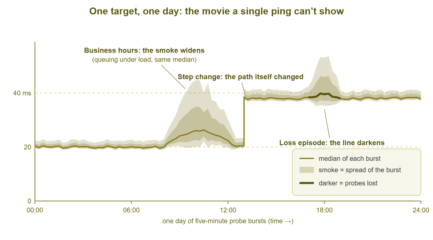
Figure 1: One target, one day. The line is the median of each burst. The gray smoke is the spread within each burst. The darker segment marks bursts that lost probes. Three of the classic patterns are visible at once.
Why the median instead of the average? Because bursts contain stragglers. If nineteen probes return in 12 ms and one wanders home in 900 ms, the average reports 56 ms. That is a number describing no packet that existed. The median calmly reports 12 ms and lets the straggler show up where it belongs: in the smoke. Averages negotiate; medians testify.
All of this is built from ping, so it inherits everything ping is and is not. Each measurement is one round trip as seen by one sender. For exactly what that number contains, see what ping actually tells you. This guide is about what happens when you stack a hundred thousand of those numbers into a picture.
Why the smoke is the genius part
Imagine two WAN circuits, both reporting an average latency of 20 ms. Circuit A delivers every packet in 19 to 21 ms, metronome-steady. Circuit B swings wildly — 5 ms, 60 ms, 8 ms, 45 ms — and merely averages 20. On an ordinary latency graph, these two circuits draw the same line. To the people using them, they are different planets. Circuit A carries a voice call beautifully. Circuit B makes calls gargle, makes remote desktop feel drunk, and generates exactly the "slow sometimes" tickets that started this article.
The difference between those circuits is jitter — the variation in delay from packet to packet. Jitter is what averages are structurally unable to show. That is the quiet genius of the smoke: it is variance made visible. A clean median line wrapped in wide, fuzzy smoke is the signature of a link that is technically fast and practically miserable. Without the smoke, that link looks healthy on every report you own.
This is the percentile thinking of measuring latency in graphical form. The median is the 50th percentile — the typical packet's experience. The upper edge of the smoke is your unlucky packets — the slow clicks and delayed keystrokes users actually complain about. An average-only graph hides precisely the packets that generate tickets; the smoke keeps them in the picture, burst after burst, forever. The smoke is where the trouble lives.
The classic patterns and what they mean
After a few weeks of watching these graphs, you stop reading numbers and start recognizing shapes, the way a radiologist reads film. Six shapes cover most of what you will ever see.
The tight, clean band
A flat median line with smoke hugging it so closely you can barely see any, in the healthy color. This is what good looks like: a path with headroom, no queuing, no drama. Nobody screenshots a healthy graph. Do it anyway. Knowing your normal median and normal smoke width for each target is the baseline every other diagnosis leans on.
The smoke that widens at business hours
The median rises a little — maybe just a few milliseconds. But the smoke blooms. It swells from 9 to 5 and calms again in the evening, flat and quiet all weekend. This is load-driven queuing: the link is busy enough that packets sometimes wait in line behind other packets. And the waiting is uneven, so the spread grows. The rhythm matching human office hours is the tell. It is not broken. It is a capacity trend wearing a costume. Watch it week over week. If the bloom starts earlier, ends later, and grows taller, you are watching a congestion problem schedule its own arrival.
The step change
The median jumps from one flat level to another — say 22 ms to 38 ms — and stays there. Latency does not settle at a new flat line for no reason. A step means something categorical changed at that moment. The traffic is taking a different path (your provider rerouted, a VPN failed over, a link in a bundle died). Or a configuration event changed how it is handled. The timestamp is the clue: correlate it with change logs, maintenance windows, and provider notices. Then compare a fresh traceroute against your old records. The guide to reading traceroute like a professional shows you how to spot where the path bent.
Spikes on a metronome
Sharp latency spikes at suspiciously exact intervals — every hour on the hour, or every night at 01:30. Nothing organic is that punctual. This is a scheduled job somewhere: a backup saturating the link, a replication run, a nightly scan, a camera system uploading footage. The backup that pings the graph, so to speak. The regularity is the fingerprint; your job is to find the scheduled task whose start time matches the spikes.
The loss-colored band
The line changes color and holds it: burst after burst is losing probes. Sustained loss is a different animal from wide smoke. The path is not just queuing packets. It is discarding them. Even a few percent makes interactive traffic feel broken (retransmissions, dropped syllables, pixelated video). A loss-colored band that comes and goes in patches is the graphical signature of the hardest fault in networking to catch by hand. The practice of hunting intermittent packet loss is a discipline of its own. And this graph is its best witness.
The gap
Nothing at all — no line, no smoke, a blank stretch of graph. Every probe in every burst vanished. Either the target went down, or the path to it died, or your monitor did. Which one? A single graph cannot say — absence of data is data, but it is ambiguous alone. This is why you graph many targets. If every graph gapped at the same moment, the monitor or its own network fell over. If one gapped while the rest stayed healthy, the problem belongs to that target. The gap teaches the golden rule of this technique: single graphs testify, but only the collection convicts.
Setting it up: the classic tool or your platform
You can get the movie two ways; both are respectable.
The original tool. Smokeping is open source, free, and has been quietly beloved by network people for a very long time. Its shape is modest. A small daemon reads a text configuration file listing your targets and probes them on schedule. It stores results in compact fixed-size database files that consolidate as data ages. It renders the graphs as simple web pages. It is happy on leftover hardware; a small Linux VM is plenty. On most Linux distributions it installs from the package manager. The real work is deciding what to watch, which is the strategy section below.
The same technique inside your monitoring platform. Most monitoring systems offer ping sensors. Many implement exactly this recipe: probe bursts on an interval, with minimum, median or average, maximum, and loss recorded and retained as history. If your platform keeps that history and can draw the spread — not just an averaged line — you get the movie in the same console as your device health and alerts. That is handy when correlating a latency step with a switch reboot.
Either path works. What you are actually shopping for is three properties — bursts, retention, and spread visualization. Any tool that provides them is doing smokeping-style graphing, whatever the name. Hold candidates to this list:
| Capability to demand | Why it matters |
|---|---|
| Probes sent in bursts, not singles | One ping is a coin flip; a burst is a sample with a shape you can graph |
| Median (not mean) as the line | One 900 ms straggler should show in the smoke, not drag the whole line |
| Spread stored and drawn | The smoke is where jitter shows; without it you own just another average graph |
| Loss painted into the same picture | Loss and latency belong together, correlated in time, not on separate charts |
| Months of per-target history | The patterns live at day, week, and month scale; a 60-minute buffer is a peephole |
| Many targets, comparable graphs | Diagnosis is reading graphs side by side; consistent scales make that instant |
| Alerting on median shifts and loss | The movie should call you when the plot turns; it should not wait to be watched |
Tip: be a polite probe citizen, and a skeptical one. Twenty pings every five minutes per target is gentle. Hundreds of targets every second is not, especially against small routers. And some devices deliberately answer ping lazily or on a quota. A scary graph can be the device's policy, not its pain. That family of deceit has its own guide, ICMP politics. Where ping is blocked outright, the same recipe works over TCP-based probes instead.
Choosing targets like a strategist
A latency graph is a statement about an entire path — every cable, switch, router, and circuit between your monitor and the target. One graph alone can only say "somewhere along this path, something happened." The strategy is to choose targets whose paths overlap in useful ways, like nested measuring sticks. When trouble comes, you diagnose by asking one question: which graphs went bad together?
Build the watchlist in tiers, each one extending the covered path by a single segment:
- Tier 1 — your default gateway. The first router your traffic touches. This graph covers only your LAN and the monitor itself; it should be the most boring picture you own.
- Tier 2 — your WAN edge. The outside of your firewall or border router. Adds your own equipment to the measured path.
- Tier 3 — the ISP's first hop. The provider router just beyond your edge (a traceroute will introduce you). Adds the last-mile circuit — the segment your provider bills you for.
- Tier 4 — one anchor per critical site or service. Each branch office router, the VPN concentrator, the data-center front door, the address of each service the business leans on — each adds one business-critical path.
- Tier 5 — one far reference point. A stable, well-run public address, such as a major public DNS resolver. This is your control group: the general internet, as seen from your seat.
The tiers nest, and the nesting is the diagnostic engine. A sick segment poisons the graph of every target whose path crosses it, and leaves every nearer graph clean. Clean near tiers exonerate; simultaneous trouble in far tiers triangulates. Two worked examples:
Scenario one: the 9:14 AM everything-hurts morning
Complaints arrive in a clump. Tier 1 (gateway): clean band. Tier 2 (edge): clean. Tier 3 (ISP first hop): smoke wide as a chimney and loss-colored since 9:05. Tier 4 (both branch anchors): same shape, same start time. Tier 5 (far reference): same again. Every path crossing the last mile went bad at once. Every path stopping short of it stayed clean. The shared segment is the ISP circuit. That is a provider ticket with graphs attached. The difference between "our internet feels slow" and "your circuit began dropping 4% of probes at 9:05, here are five independent graphs" is the difference between a shrug and an engineer.
Scenario two: one branch, one bad graph
Branch B's anchor stepped up 40 ms at 2:00 AM and stayed there. Its smoke looks normal, just relocated upstairs. Every other graph — gateway, edge, ISP hop, branch A, far reference — is untouched. Every shared segment is exonerated. The cause lives on the path only branch B's probes travel. A step at exactly 2:00 AM smells like a maintenance window or an automatic failover — the branch VPN re-homing to a backup circuit, say. Run a traceroute to branch B and compare it with your notes from last week. The hop where the paths diverge is your answer.
One honest limitation: every graph shares the monitor's vantage point. Trouble on the monitor's own switch dirties everything at once, and some asymmetries are invisible from one side. A second probe location — say, a small probe at a branch graphing the path back toward headquarters — breaks those ties. The placement craft is covered in designing synthetic probes.
Retention and granularity
Two dials matter: how often you burst, and how long you keep the results. Five-minute bursts are the classic default and right for most targets. For a critical WAN link you may drop to one minute — problems shorter than your interval can slip between bursts. Below one minute, returns diminish: more probe traffic and more noise, for little the one-minute view missed.
Retention has a subtlety. Nobody keeps every burst at full detail forever. Storage systems consolidate old data into coarser summaries. The trap is how they consolidate. If old data is reduced to averages of averages, the smoke evaporates. Last month's jittery afternoon flattens into a serene line, and history quietly lies to you. Good implementations carry maximums or percentiles through consolidation so old data keeps its spread. Check yours before you need history as evidence, because that is exactly when you will discover the smoke is gone.
Keep a long history — a year if you can. This data is tiny. A burst summary is a handful of numbers. There are roughly a hundred thousand bursts per target per year at five-minute intervals, which is trivial storage. What a year buys you is rhythm: month-end closes, seasonal load, the slow widening of business-hours smoke. That widening tells you a circuit upgrade belongs in next year's budget rather than next quarter's emergency.
The longest-term payoff is the least technical. After a few months, "normal" stops being a number you look up and becomes a shape you recognize. And your eye will snag on the one wrong graph before you can say why. That reflex cannot be installed — only grown, five minutes at a time.
Your five-target starter watchlist
Enough theory. Set up five targets tonight:
- 1. Default gateway — proves your LAN and the monitor itself.
- 2. WAN edge (firewall or border router) — proves your own equipment.
- 3. ISP first hop — proves the last-mile circuit.
- 4. Your most critical remote anchor (main branch, data center, or VPN endpoint) — proves the path the business feels first.
- 5. A far reference point (a major public resolver) — proves the general internet, as your control.
When something goes wrong, read across all five and use the correlation table:
| Graphs that went bad together | Where the problem lives | First move |
|---|---|---|
| All five at once, including the gateway | Your LAN or the monitor itself | Check the monitor's own host and switch before blaming any network |
| Everything except the gateway | Your WAN edge device or its uplink | Check firewall CPU, sessions, and the edge port counters |
| ISP hop and everything beyond it; tiers 1–2 clean | The last-mile circuit | Open a provider ticket with the graphs attached |
| One remote anchor only; all else clean | That site or its specific path | Traceroute toward it; check its VPN, circuit, and local kit |
| Far reference only; all anchors clean | Distant internet weather | Usually not actionable; note it and resist heroics |
| Gaps on every graph simultaneously | The monitor died, not the network | Revive the monitor; apologize to nobody |
Where to go next
The recipe once more: bursts of probes to strategic targets, forever; median as the line, spread as the smoke, loss as the color. The smoke shows the jitter that averages hide. The patterns turn shapes into diagnoses. And the tiered watchlist turns a wall of graphs into a triangulation instrument. "Slow sometimes" stops being a mystery and becomes a timestamped, screenshot-able fact.
A natural next step in this topic is MTR — the portable cousin of this technique. It probes every hop along one path continuously during a live investigation. Smokeping-style graphs are the permanent record of the ends. The rest of the Ping, Traceroute & Friends guides cover the tools and the politics around them.
Put this into practice with SysPeep Monitor
Continuous graphs only work if something tireless draws them. SysPeep Monitor is built for that kind of stamina. It runs on one Windows machine and auto-discovers your devices. It collects health and performance metrics around the clock, and alerts you the moment answers change for the worse. Its dashboards put your graphs and your device status side by side. The free trial takes minutes to install.
Download Free TrialLearn About SysPeep - All Rights Reserved.