
The Four Delay Types: Propagation, Serialization, Queuing, Processing
Every millisecond of network delay you will ever measure — every ping time, every laggy remote session, every "why is this 80 ms?" — is made of exactly four ingredients. Not five, not a mysterious continuum: four. A packet crossing a network spends its life doing only four things. It travels down wires, squeezes onto links one bit at a time, waits in line inside devices, and is thought about by those devices. Each of those has a name, a formula you can do in your head, and — this is the payoff — a completely different fix. One of them has no fix at all.
That last sentence is why this taxonomy is worth an hour of your life. Suppose latency is hurting and someone proposes a cure — a bandwidth upgrade, a shiny new firewall, a quality-of-service project. The four types tell you instantly whether that cure can even touch the disease. This guide walks through each type with the physics made friendly. It gives you the formula in plain words and worked numbers you can check on a calculator. It gives an honest verdict on what, if anything, you can do about it. By the end you will be able to look at a latency number and ask the only question that matters. That question is: which of the four is this, and do I own a lever that moves it?
In this guide
- Why bother naming delays?
- Propagation: the distance tax
- Serialization: the doorway tax
- Queuing: the waiting room
- Processing: the device think-time
- Adding it up: a delay budget for one real path
- The verdict table: which lever helps
- Where to go next
Why bother naming delays?
When you measure a round-trip time, you measure the out-and-back travel time. The round-trip anatomy guide establishes that as the currency of all latency work. You get one number: say, 48 ms. That number is a sum. Every link and every device between you and the target contributed a pinch of each of the four delay types, in both directions. The pinches added up to 48. The trouble with a sum is that it hides its ingredients. A 48 ms path that is mostly distance is perfectly healthy and permanently unfixable. A 48 ms path that should be 12 ms but is drowning in queuing is sick and very fixable. Same number, opposite meanings.
The four types are the decoder. Two of them — propagation and serialization — are fixed physics. They depend on distance and link speed. They produce the stable floor under every measurement, the number your path simply cannot go below. One — queuing — is the volatile ingredient: it is zero on a quiet network and huge on a congested one. And it is responsible for nearly all of the moment-to-moment variation you see. The last — processing — lives inside boxes with CPUs and configurations, which means it lives inside things you administer. Those stories are floor, variance, and overhead. Once you can split a latency number into those three stories, you know which team, which purchase, or which law of physics you are negotiating with.
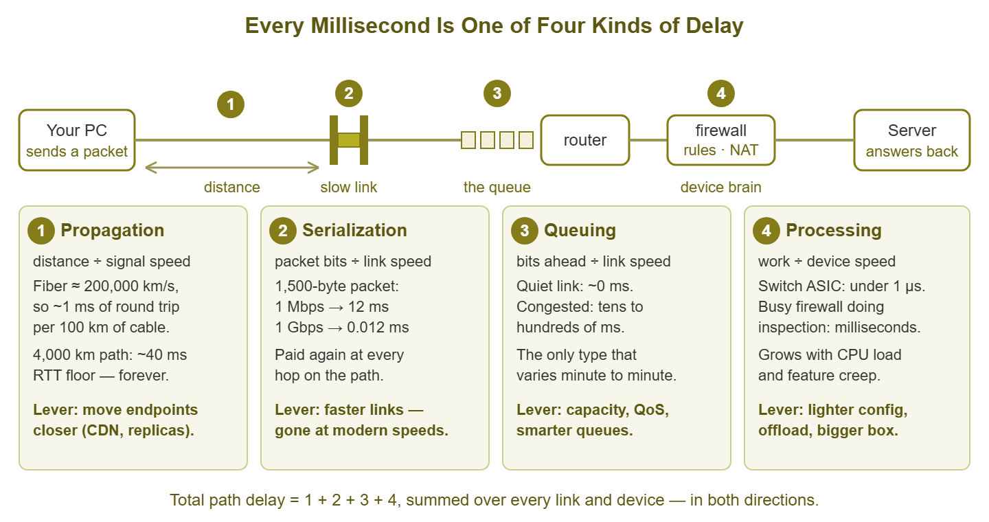
Figure 1: The four places a packet spends time. Total path delay is the sum of all four, collected at every link and device, in both directions.
Propagation: the distance tax
What it is: the time the signal spends physically traveling along the medium — light in a fiber, electrons in copper, radio through air. The formula in plain words: distance divided by the speed of the signal. Nothing else appears in that formula. Not the price of the router, not the bandwidth of the link, not the vendor. Distance and the speed of light: that is the whole equation.
The speed part is worth knowing cold. In a vacuum, light travels about 300,000 km per second. Inside glass fiber it travels slower — roughly two-thirds of that, about 200,000 km per second, because it is constantly refracting through the glass. Signals in copper move at a broadly similar fraction. That gives you a rule of thumb worth memorizing: about 1 ms of one-way delay per 200 km of cable — so about 1 ms of round-trip time per 100 km. Now work the ladder:
| Path | Cable distance | One-way propagation | Round trip |
|---|---|---|---|
| Patch cable to the switch | 3 m | 0.000015 ms | 0.00003 ms |
| Across a campus | 2 km | 0.01 ms | 0.02 ms |
| Metro fiber across a city | 80 km | 0.4 ms | 0.8 ms |
| Cross-country fiber route | ~4,000 km | ~20 ms | ~40 ms |
| Intercontinental route | ~12,000 km | ~60 ms | ~120 ms |
| Geostationary satellite (up + down) | ~71,600 km through space | ~239 ms | ~478 ms |
Two honest footnotes on that table. First, fiber routes are not straight lines. They follow railways, roads, and seabeds, and they detour through cities. So the real cable distance between two places is comfortably longer than the map distance. A coast-to-coast path with a ~40 ms theoretical round-trip floor typically measures 60 to 70 ms in real life once route wander and equipment are included. Second, the satellite row uses the full speed of light, because radio in space is not slowed by glass. The delay is still enormous, because a geostationary satellite parks about 35,786 km above the equator. Your packet must climb all the way up and come all the way down just to reach the ground station.
Can you fix it? No. This is the type with no fix, and it deserves to be said plainly. The rule is: no product, no budget, and no vendor can reduce propagation delay on a given path. The alternative is speeding up light. A cross-country link has a hard floor of several tens of milliseconds round trip, forever. What you can do is refuse to pay the tax so often: move the endpoints closer together. That is the entire intellectual content of a content delivery network (CDN). That service keeps copies of content in many cities so users fetch from a nearby copy. The same idea underlies regional server replicas, branch-side caches, and "put the app where the users are" architecture decisions. You cannot shorten the road; you can move the destination.
Serialization: the doorway tax
What it is: a network link transmits one bit at a time, in order. Before a packet can travel anywhere, the sending device must clock every bit of it out onto the wire. It is like a crowd filing through a doorway single file. Serialization delay is the time that takes. The formula in plain words: the packet's size in bits, divided by the link's speed in bits per second. A bigger packet or a slower door means a longer wait. And the toll is charged again at every hop along the path. Each device receives the packet and then must clock it out again onto the next link.
Work the numbers for the internet's most common packet, a full-size 1,500-byte frame, which is 12,000 bits:
| Link speed | Time to serialize one 1,500-byte packet | Feels like |
|---|---|---|
| 1 Mbps | 12 ms | A real, human-noticeable delay per packet |
| 10 Mbps | 1.2 ms | Small but measurable |
| 100 Mbps | 0.12 ms | Background noise |
| 1 Gbps | 0.012 ms | Irrelevant |
| 10 Gbps | 0.0012 ms | Deeply irrelevant |
The table tells the whole story: serialization is a big deal on slow links and a rounding error on fast ones. On a 1 Gbps office LAN you will never think about it. But on a slow WAN uplink, a strained VPN over weak residential upload, or an aging leased line, it bites — and it bites unfairly. Picture a small voice packet stuck behind a full-size download packet on a 1 Mbps link. The voice packet waits 12 ms just for the fat packet ahead of it to clear the doorway. That happens at every such hop, in addition to all its other delays. (Old-timers will remember elaborate tricks for fragmenting big packets on slow serial links precisely to spare voice traffic this fate. Faster links made most of those tricks museum pieces.)
Can you fix it? Yes, and the fix is refreshingly blunt: faster links. Every step up the speed ladder divides the doorway tax by ten. This is one of the few latency problems that a bandwidth upgrade genuinely solves. That is worth savoring, because the latency vs. bandwidth guide is largely a catalog of latency problems that bandwidth upgrades do not solve. If your slowest link is already 100 Mbps or better, serialization is almost never your story.
Queuing: the waiting room
What it is: when packets arrive at a device faster than the outgoing link can send them, the device does not throw them away (not immediately, anyway). Instead, it parks them in a memory buffer, a waiting line for the doorway. Queuing delay is the time a packet spends standing in that line. The formula in plain words: how many bits are ahead of you in the queue, divided by the speed of the link you are all waiting for. A queue of twenty full-size packets on a 100 Mbps link is twenty times 0.12 ms — about 2.4 ms of added delay. The same queue on a 10 Mbps link is 24 ms. Queuing is serialization's revenge: every packet ahead of you charges you its own doorway time.
Queuing has a property none of the other three types share: it changes from moment to moment. Propagation is constant. Serialization is constant for a given packet size. Processing is roughly constant until a device is overloaded. But queues live and die with traffic: empty at 2 AM, modest at 10 AM, savage during the Friday backup window. Suppose users say the network is "sometimes slow." Or your latency graphs show spikes at the same hours every day. Or a ping that is usually 12 ms occasionally reads 180 ms. When you see that variability, it is queuing, essentially always. It is the signature.
The relationship between queuing and utilization is viciously nonlinear. A link at 50% busy has short lines that clear instantly. At 90%, lines form and linger. As utilization approaches 100%, queue length — and therefore delay — grows explosively. That is because packets arrive about as fast as they can possibly leave and every burst piles up. This is why a link can be "not full" on the five-minute average graph and still be a latency disaster during one-second bursts. And buffers are oversized in a depressing amount of consumer and edge equipment. When they are, a saturated link can hide hundreds of milliseconds of standing queue. That can ruin every interactive application that shares it. That failure mode is common enough to have earned its own name and its own guide: bufferbloat.
Can you fix it? Yes — queuing is the most fixable of the four, which is fortunate since it causes most of the pain. Here are the levers, in rough order of how often they are the right answer. Add capacity so the queue never forms (a genuinely faster bottleneck link). Give latency-sensitive traffic priority boarding with quality of service (QoS), so voice and interactive packets jump the line that bulk transfers built. And use smarter queue management — modern buffer disciplines that keep lines deliberately short instead of letting them grow. The bufferbloat guide shows these transforming a link. The prerequisite for all three is knowing which link is queuing, which is a monitoring question: watch utilization and watch latency, together, over time.
Processing: the device think-time
What it is: every device that handles a packet spends some time deciding what to do with it. That work includes reading headers, looking up where the destination lives, and rewriting addresses for NAT (network address translation). It includes checking the packet against firewall rules, inspecting it for threats, and encrypting or decrypting it for a VPN. Processing delay is that think-time. The formula in plain words: there is no tidy formula. It is the work the device does per packet, divided by how fast its silicon can do that work. That is exactly why it varies so much between boxes.
The range is wide but the pattern is simple. A switch forwarding frames in dedicated hardware (an ASIC — a chip built to do one job absurdly fast) thinks in well under a microsecond. You will never see it on a graph. A router doing ordinary lookups in hardware is similar. But move the work onto a general-purpose CPU and start piling on features — long rule lists, deep packet inspection, antivirus scanning, VPN cryptography. Think-time then climbs into fractions of a millisecond, then whole milliseconds. Now load that CPU to its limit during the morning rush and think-time stops being constant. In that case, packets wait not for a link, but for the processor itself. Latency through the box swells and jitters. A firewall at 95% CPU is a latency problem you can see coming a week away — if you are watching device CPU at all. The same logic applies in miniature to a home-grade router doing NAT for a too-busy household, and at the endpoints too. A swamped server adds its own think-time before its network stack even answers.
Can you fix it? Yes, in three escalating ways. Lighten the work: prune rule lists, and disable inspection features nobody consciously chose for traffic that does not need them. Make sure high-volume flows take the device's hardware fast path instead of the CPU path. Watch the load: device CPU and memory are standard SNMP metrics. And a climbing trend is your early warning (the free-tools measurement guide shows how to collect them). And when the work is legitimate and the box is simply too small for it: better hardware. Processing delay is the one type you can literally buy your way out of — as long as it was actually processing delay. That is the whole reason to diagnose before purchasing.
Adding it up: a delay budget for one real path
Now assemble a realistic path and watch the four types claim their shares. A user's PC in a branch office reaches a server 1,200 km away. The path goes through the branch LAN (two switch hops at 1 Gbps) and the branch firewall (doing NAT and inspection). It continues through a 100 Mbps WAN uplink, the long-haul fiber, and the data-center LAN on the far side. Here is the round-trip budget on a quiet morning versus a congested afternoon:
| Delay type | Quiet (round trip) | Congested (round trip) | Where it accrued |
|---|---|---|---|
| Propagation | ~12 ms | ~12 ms | The 1,200 km of fiber, both directions |
| Serialization | ~0.3 ms | ~0.3 ms | Every hop; almost all of it at the 100 Mbps uplink |
| Queuing | ~0.4 ms | ~85 ms | The WAN uplink's buffer during the afternoon crunch |
| Processing | ~1.3 ms | ~3 ms | Firewall inspection; its CPU is busier at 2 PM |
| Total RTT | ~14 ms | ~100 ms | Same path, same gear, different hour |
Read the table twice, because it contains the two most useful facts in latency troubleshooting. First: the floor is propagation. On the quiet morning, distance is roughly 85% of the total; the fancy equipment contributes crumbs. Whenever a path is at its floor, it is healthy, and the only way to a lower number is a shorter path. Second: the variance is queuing. Between morning and afternoon, three rows barely moved; one row grew two hundred times. When a path's latency varies with the clock or with load, you are hunting a queue. In that case, the hunt is to find which link's buffer it is.
Tip: next time a vendor or a colleague promises that some purchase will "cut latency," ask the four-types question out loud: which type? If the path's delay is mostly propagation, the honest answers are relocation, caching, or acceptance — not hardware. If it is queuing, capacity and QoS are on the table. The question takes ten seconds and has saved organizations from some very expensive placebos.
The verdict table: which lever helps
The whole guide, in one artifact. When a latency number bothers you, identify the type, then look up your lever:
| Type | Plain-words formula | Typical size | Varies moment to moment? | Your levers |
|---|---|---|---|---|
| Propagation | Distance ÷ signal speed | ~1 ms RTT per 100 km | No — it is the floor | None on the path itself. Move endpoints closer: CDN, regional replicas, caches |
| Serialization | Packet bits ÷ link speed | 12 ms at 1 Mbps → 0.012 ms at 1 Gbps | No (per packet size) | Faster links; vanishes at modern speeds |
| Queuing | Bits ahead of you ÷ link speed | 0 when quiet; tens to hundreds of ms when congested | Yes — the only one | Capacity at the bottleneck, QoS priority, smarter queue management |
| Processing | Work per packet ÷ device horsepower | Sub-µs in a switch ASIC; ms in a loaded firewall | Somewhat, with device load | Lighter config, hardware fast path, right-sized hardware |
And here are the diagnostic shortcuts, which are really just the table read sideways. A latency floor that never goes lower no matter the hour is propagation. Check whether it matches the distance before declaring it a problem (the baselines guide gives reference ranges per path type). Latency that swells with load or time of day is queuing. Latency that steps up at one specific device — and tracks that device's CPU graph — is processing. And a slow link with big packets, in the rare places those still exist, is serialization. Four signatures, four investigations, no guessing.
Where to go next
You now know what a millisecond is made of — and, more importantly, which milliseconds are negotiable. The floor belongs to physics; the spikes belong to queues; the overhead belongs to boxes you configure. To see these four types priced into a whole application click — handshakes, server think-time and all — read the anatomy of a round trip. To know what total delay is normal for a given kind of path, keep the latency baselines reference within reach. And when you are ready to chase a real problem through a real network, the high-RTT troubleshooting guide turns this taxonomy into a decision tree. The full collection lives on the Network Latency pillar page.
Put this into practice with SysPeep Monitor
Two of the four delay types leave fingerprints a monitoring system catches early. Queuing shows up as response times drifting with load. Processing shows up as climbing CPU on a firewall or router. SysPeep Monitor collects both around the clock: device health over SNMP and WMI, response-time graphs for every path you care about. It alerts you when today stops looking like your normal. The free trial installs on a Windows machine in minutes.
Download Free TrialLearn About SysPeep - All Rights Reserved.