
Capacity Planning for People Who Have Never Done It
Something on your network is going to fill up this year. A disk, a link, a licence count, a block of switch ports. You do not know which one yet, and that is the whole problem. The first you hear of it will be a ticket, a stalled backup, or a user who cannot get an address. Capacity planning is the habit of finding out months earlier, from data you are already collecting, and doing something about it before anyone notices.
This guide assumes you have never done it. Every term is defined where it appears. The arithmetic stays at subtraction and division. And there is a one-table register you can fill in this afternoon. By the end you will know what capacity and headroom mean and which four kinds of resource fill up. You will know why your monitoring history is the only input worth trusting. You will also know how to run the five-step loop that turns a graph into a purchase order before the pain starts.
In this guide
- What capacity actually means
- Headroom and lead time, defined plainly
- The four things that fill up
- Why monitoring history is the only honest input
- The loop: measure, project, decide, buy, verify
- How much history you need
- Who owns the plan
- A starter capacity register
- The file server that filled on a public holiday
- Checklist
- Where to go next
What capacity actually means
Capacity is how much of a resource you have, compared with how much of it you are using, tracked over time. All three parts matter. "How much you have" is the limit: a two-terabyte volume, a one-gigabit link, a forty-eight-port switch, a licence for two hundred devices. "How much you use" is the current reading from monitoring. "Over time" is the part people skip, and it is the part that makes this planning rather than a snapshot.
A snapshot tells you the state; the trend tells you the future. A volume at seventy percent is fine if it has sat at seventy percent for two years. The same volume is an emergency if it was at fifty percent in the spring. The number is identical and the story is opposite. Everything in this pillar is about reading the story, not the number.
The analogy I use is the fuel gauge. The gauge tells you the tank is half full. Useful, but it does not tell you whether to stop. For that you need to know how fast the needle is falling and how far it is to the next station. Capacity planning is the same three questions: how much is left, how fast is it going, and how long until I can get more.
Headroom and lead time, defined plainly
Headroom is the gap between what you use and what you have. If the volume holds two terabytes and you have used one and a half, your headroom is half a terabyte. Headroom is measured in the resource's own units first and in time second. Half a terabyte of headroom is a comfortable year if you add forty gigabytes a month. It is a nervous three months if you add a hundred and seventy.
Lead time is how long it takes to get more. Measure it from the moment you decide you need it to the moment it is in service. Not the moment it is delivered; the moment it is doing the job. A new circuit that arrives in six weeks and then waits a month for a cutover window has a ten-week lead time. Lead time is the number most junior admins have never asked about and most purchasing teams have never been asked. (Both sides are quietly surprised by it.)
The whole discipline fits in one sentence: you must notice that headroom is running out at least one lead time before it does. Everything else is technique for noticing earlier and stating it convincingly. The guide on lead time and buying before the pain walks the purchasing chain step by step. For now, hold on to the idea that "how long to get more" is a number you need for every resource you care about.
The four things that fill up
Almost every capacity problem on a network is one of four kinds, and it helps to name them. They fill at different speeds, they are measured in different ways, and they hurt differently when they run out.
Bandwidth
Bandwidth is the carrying capacity of a link, measured in bits per second. A link "fills" when the traffic offered to it approaches its speed for long enough that packets queue up and users feel the wait. Bandwidth is the resource most people think of first, and it already has its own guides. The guide how full is too full covers the queuing behaviour. And utilisation to purchase timing covers reading the graph to time a circuit order.
Storage
Storage is disk space: server volumes, backup targets, the datastore under your virtual machines, and the database your monitoring system writes into. It fills in a straight line more often than anything else, and it is the resource with the fewest excuses. The trend is visible on any graph a year long. A full disk is also the most decisive failure of the four. Services do not slow down; they stop.
Compute and memory
Compute and memory are the processor time and RAM on your servers, including the monitoring server itself. These fill in a different pattern. They do not climb steadily so much as get busier at the peak, until the busy hour becomes the busy afternoon. "Full" here means the peak reaches a level where work queues up, not a hard wall. Plan them on the busy-hour maximum, never the daily average. An average CPU of thirty percent can hide an hour a day at ninety-five.
Slots
Slots are things you count rather than measure. These include switch ports, IP addresses in a subnet or a DHCP scope, licences, rack units, PoE watts, UPS outlets. A slot is either taken or free. Slots fill in steps, one project at a time, and they are the ones that surprise people because nobody graphs them. The guide on capacity beyond bandwidth goes through each of them, with the counter or check that gives you the number.
You will notice that only one of the four is bandwidth. A capacity plan that stops at the WAN link is a plan for a quarter of the outages.
Why monitoring history is the only honest input
The only trustworthy input to a capacity plan is the record of what actually happened. Not the vendor's sizing guide, not last year's project forecast, not the number of users someone quoted in a meeting. Those are all opinions about the future. A year of monitoring samples is a fact about the past, and the past is the only thing anyone has measured.
Growth comes from behaviour, and behaviour is invisible until it is recorded. Nobody planned for the scan-to-email habit that doubled the file server's growth. Nobody wrote a project plan for the department that discovered it could keep meeting recordings forever. The monitoring history saw all of it, because the monitoring history saw the disk.
This is why a monitoring system that keeps long-term history is worth more for planning than any amount of estimating. If yours throws samples away after ninety days, you have a very good alarm clock and no calendar. The guide on rollups and retention explains how monitoring data ages into summaries. The summary you need for planning is the daily peak, kept for at least a year.
The loop: measure, project, decide, buy, verify
Capacity planning is a loop of five steps, and it runs continuously rather than once. Here is each step in a sentence, then the detail.
- Measure: record the current use and the limit for each resource, from monitoring, on a fixed day each month.
- Project: extend the trend forward and estimate the date the resource reaches its limit.
- Decide: compare the projected full date with the lead time and choose to buy, shrink, or wait.
- Buy: start the purchase early enough that the new capacity is in service before the projected full date, with margin.
- Verify: after the change, confirm from monitoring that headroom really did increase, then return to step one.
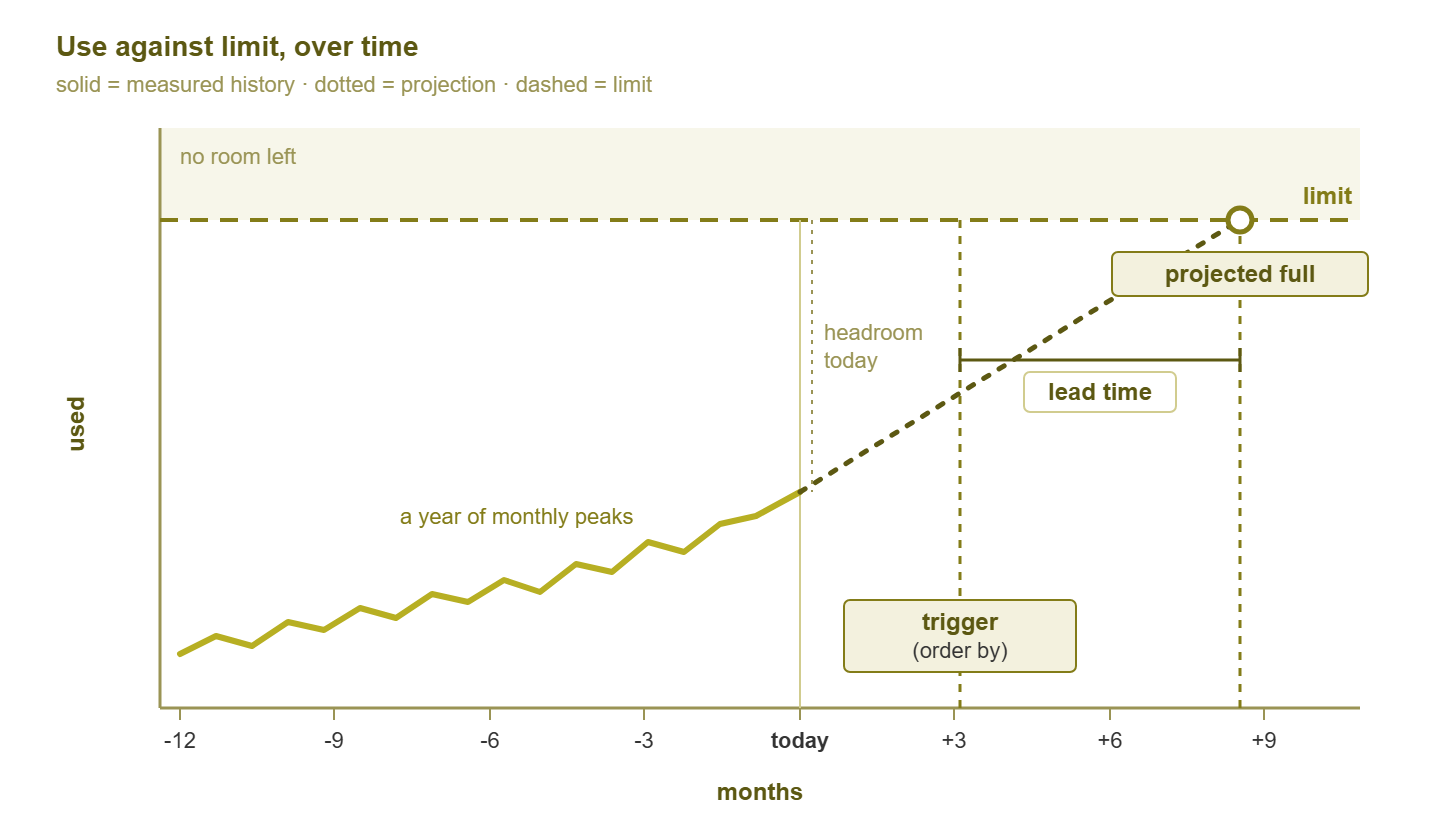
Figure 1: The whole method on one graph. The trend line is the past. The dotted line is the projection. And the trigger sits one lead time (plus a margin) before the crossing.
Measure means reading the number off the monitoring system, not guessing it. For a volume that is used bytes and total bytes. For a link it is the busy-hour peak utilisation for the month. For a licence it is the count of devices consuming one against the count purchased. Write it in the register with the date. If you want the disk numbers from a Windows host directly, one line of PowerShell gives you used and total per volume:
Get-CimInstance Win32_LogicalDisk -Filter "DriveType=3" |
  Select-Object DeviceID,
    @{n='UsedGB';e={[math]::Round(($_.Size-$_.FreeSpace)/1GB,1)}},
    @{n='SizeGB';e={[math]::Round($_.Size/1GB,1)}}
Project means drawing a line. In its simplest form you take the reading from twelve months ago and the reading today. Divide the difference by twelve to get growth per month. Then divide the remaining headroom by that growth. Three lines of arithmetic, and they are the same three lines for a disk, a link, or a licence count:
growth per month = (use today - use 12 months ago) / 12
months to full   = (limit - use today) / growth per month
projected full   = today + months to full
Here it is worked once with example numbers. A volume at 1,620 GB today that was at 1,080 GB a year ago has grown 540 GB in twelve months. That is 45 GB a month. Its limit is 2,000 GB, so headroom is 380 GB, and 380 divided by 45 is a little over eight months. That is the projected full date, give or take the seasonal effects the forecasting guide deals with.
Decide is where you apply the lead time. If the projected full date is eighteen months out and the lead time is two, you write it down and move on. If it is five months out and the lead time is four, you start the purchase this week. Decide also includes the option nobody remembers: shrink. Deleting the four terabytes of old installer images is a capacity project with a lead time of one afternoon. (It also produces an email thread with a lead time of several weeks.)
Buy is the slow step, and the one you control least. Its length is the lead time and its start date is the trigger. Start it at the trigger, not when the graph turns red. By the time the graph turns red the lead time has already been spent.
Verify closes the loop, and it is the step people skip. After the new disk is in, the next monthly reading should show that headroom jumped. If it did not, the migration did not finish, the wrong volume was extended, or growth accelerated the moment space appeared. All three happen. The graph will tell you which.
How much history you need
A full year, if you can get it. Use is seasonal in ways you do not expect, and a year is the shortest window that contains every season once. It has the year-end close, the summer lull, and the intake of new starters. It also has the annual audit that copies everything twice, and the one week every department decides to tidy its shared drive. The guide on seasonal patterns catalogues these rhythms. For planning, you only need to know that they exist and that a short window hides them.
A quarter lies. Draw a trend line through three months and you are projecting whatever those three months happened to contain. Three quiet summer months give you a flat line and a false sense of security. Three months containing a migration give you a cliff. I once sized a backup target on a spring quarter that included a one-off archive import and ordered twice what we needed. The finance team remembers this more clearly than I would like.
If you do not have a year yet, plan with what you have and say so. Write "based on four months of data" on the register and on any proposal. Six months is much better than three. Three is much better than a vendor's sizing formula. And any monitoring history is better than the memory of the person who set the server up. Meanwhile, keep collecting. The plan gets more honest every month.
One caution about what "history" means. Monitoring systems store detail for recent days and summaries for older ones. The summary for a day may be the average, the maximum, or both. Plan from the daily maximum where it is kept. The average underestimates every peak-driven resource, and "we planned on the average" is not a sentence you want to say in the review. If you already keep a baseline (the recorded normal for a metric), the planning data is already there.
Who owns the plan
Someone has to own the register, or nobody looks at it. In a small team that is you, and the job is one hour on the first working day of each month. Update the readings and recompute the projections. Flag any resource whose trigger date falls inside the next quarter, and send the list to whoever approves spending. The monitoring data for management pillar covers how to present that list so it gets read.
Ownership is a name, not a department. "The infrastructure team" owns nothing; a person with a calendar reminder owns something. The plan should also have a second reader, someone who sees the register once a quarter and asks the questions the owner has stopped asking. An hour a month and a reader who is not you. That is the entire governance structure.
Tip: put the monthly update in your calendar as a recurring appointment, and put the register's file path in the appointment title. The reminder that says "capacity" gets dismissed. The reminder that says where the file is gets opened.
A starter capacity register
The register is one table, and it lives in a shared file that survives you. Each row is one resource. Eight columns. Here is the template with example rows filled in so you can see the shape; every number is invented for the example.
| Resource | Current use | Limit | Trend per month | Projected full | Lead time | Trigger date | Owner |
|---|---|---|---|---|---|---|---|
| fs01.example.com volume D: | 1,620 GB | 2,000 GB | +45 GB | 8 months out | 6 weeks | 5 months out | J. Ortiz |
| Head office WAN link | 71% busy-hour peak | 100% of 100 Mbit/s | +2 points | 14 months out | 12 weeks | 10 months out | J. Ortiz |
| Core switch access ports | 44 used | 48 | +1 port | 4 months out | 3 weeks | 2 months out | M. Adeyemi |
| Monitoring device licences | 186 | 200 | +3 | 5 months out | 2 weeks | 3 months out | J. Ortiz |
| DHCP scope 10.20.0.0/22 | 790 leased | 1,000 usable | +15 | 14 months out | 1 week | 12 months out | M. Adeyemi |
How to fill each column, once per row:
- Resource: name it exactly as the monitoring system names it, so the next person can find the graph.
- Current use and limit: the same units in both columns. Bytes with bytes, ports with ports, percent with percent.
- Trend per month: the change per month over the last year of data, from the formula above.
- Projected full: headroom divided by trend, written as a month.
- Lead time: what procurement told you, with the date they told you.
- Trigger date: projected full, minus lead time, minus a safety margin of at least one month.
- Owner: a person's name.
Five rows is a fine start. Add a row whenever something fills up that was not on the list. The register will be complete in about a year, which is also how long it takes to become useful. The guide on justifying an upgrade with graphs turns any one row into a proposal.
The file server that filled on a public holiday
Meridian Parts had a file server, fs01.example.com, that had been "at about eighty percent" for as long as anyone could remember. Everyone took the steadiness as reassurance. Nobody had opened the year-long graph, which showed a straight line climbing roughly fifty gigabytes a month since the scanning project started. The line crossed one hundred percent at two in the morning on a public holiday. The nightly backup failed to write its log. The order system that kept its export files on the same volume stopped exporting. The first person to notice was a customer, on the first working day, asking where the invoices were. The replacement disk took a week to order and an afternoon to install. The graph had been predicting the date for nine months.
Every part of that story is ordinary. The steady number was a real reading. The straight line was a real trend. And the public holiday was just the day the arithmetic finished. What was missing was the loop. Nobody measured on a fixed day, so nobody projected, so the purchase started after the pain instead of before it.
Checklist
- List every resource that would cause an outage if it filled: volumes, links, ports, scopes, licences, power, and memory on key hosts.
- Confirm the monitoring system keeps at least a year of daily-peak history for each one; if not, change the retention now.
- Fill in the register with today's readings and limits, in matching units.
- Compute the trend per month from the oldest and newest readings you have, and note how many months of data it rests on.
- Ask procurement for the lead time of each kind of resource and record the answer.
- Set a trigger date for each row: projected full, minus lead time, minus one month.
- Name an owner and put the monthly update in the calendar.
- Add a monitoring threshold at the utilisation level that corresponds to each trigger, so the register is backed by an alert.
- After every upgrade, verify from the graph that headroom actually increased.
Where to go next
You now have the vocabulary and the loop. Capacity is use against limit over time. Headroom is the gap. Lead time is how long the gap takes to close from your side. The register is where the three meet once a month. The rest of Capacity Planning From Monitoring History takes each step further. It covers projecting the trend with a ruler and a spreadsheet, and finding the real lead time and setting the trigger. It also covers the resources beyond bandwidth that fill up unannounced and the one graph that gets an upgrade approved. Start with the register. Everything else improves a column in it.
Put this into practice with SysPeep Monitor
A capacity register is only as good as the history behind it. SysPeep Monitor keeps long-term graphs and reports in one web console. It lets you set thresholds on utilisation so a trigger point arrives as an email rather than a surprise. It stores the history in SQLite, MySQL/MariaDB, or SQL Server so it is still there when planning day comes round. The free trial installs on any Windows machine.
Download Free TrialLearn About SysPeep - All Rights Reserved.